1 Toolkit for network analysis

Alessandro Vindigni
session 14/03/2024

An ecological network is a dataset describing a group of species and their reciprocal interaction. Typically, this data is collected by ecologists in the field, even if for some purposes ecological networks can also be generated by computer simulations. In recent publications experimental datasets are usually made available, either as supplemental material or through a repository on the web. Some research groups have also gathered network datasets from different publications into public databases to facilitate access to the scientific community. Two of such examples are Mangal and Web of life.

In this session you will learn how to download datasets from the Web of life database of experimental ecological networks and convert them into several formats that are suitable for analysis. Finally, we will compute one network property – the connectance – and plot it.

1.1 The web of life

Web of life is a database of ecological networks developed and maintained by the Bascompte lab. More information about the project can be found in this paper, while here you can find a manual to download ecological networks manually. In this section you will learn to automate downloading the networks available on web of life, visualize them, and perform some basic calculation using those data.

This web interface provides a visualization of where data of a given network have been collected over the globe. Clicking the dot corresponding to a network, the relative metadata can be visualized as well as a 3D representation of the network. The incidence matrix is also displayed and can be downloaded in different formats.
Networks are named according to the following convention

interaction type: mutualistic (M) or antagonistic (A)
network type: Plant-Ant (PAO), Plant-Epiphyte (PE), Pollination (PL), Seed Dispersal (SD), Food Webs (FW), Host-Parasite (HP), Host-Parasitoid (HPD), Plant-Herbivore (PH), Anemone-Fish (AF)
id labeling a specific network.

1.1.1 Download one network from the weboflife API

In a research projects it is often convenient to bypass the web interface and store data directly in a dataframe using a command line. This has several advantages in terms of efficiency and reproducibility of the analysis you are conducting. We will see how to do this in R using the function fromJSON() of the package jsonlite, but similar commands can be run in python or in other languages. To this aim, we have opened few dedicated endpoints on the Application Programming Interface (API) of the web-of-life project.

Let us focus on the network number 002 of the Seed Dispersal type, named M_SD_002: the set of commands to download it are

# define the base url
base_url <- "https://www.web-of-life.es/"     
# define the full url associated with the endpoint that download networks interactions
json_url <- paste0(base_url,"get_networks.php?network_name=M_SD_002")
# import the jsonlite package (if not done at the beginning) 
library(rjson) 
# and run it 
M_SD_002_nw <- jsonlite::fromJSON(json_url)
class(M_SD_002_nw$connection_strength) <-"numeric"

It is always good practice to have a look at the class of a newly defined object (dataframe) and display its first rows to understand how this data looks like, number of columns, their names, etc.

# check the class 
class(M_SD_002_nw)

## [1] "data.frame"

# have a look at the dataframe
head(M_SD_002_nw)

##   network_name                 species1              species2
## 1     M_SD_002        Cissus hypoglauca Manucodia keraudrenii
## 2     M_SD_002                Ficus gul Manucodia keraudrenii
## 3     M_SD_002            Ficus odoardi Manucodia keraudrenii
## 4     M_SD_002 Chisocheton sp1 M_SD_002 Manucodia keraudrenii
## 5     M_SD_002   Dysoxylum sp1 M_SD_002 Manucodia keraudrenii
## 6     M_SD_002 Elmerrillia sp1 M_SD_002 Manucodia keraudrenii
##   connection_strength
## 1                  13
## 2                 155
## 3                  55
## 4                   7
## 5                   1
## 6                   8

The content of a dataframe can be visualized more nicely using the package formattable

# import the dplyr package (if not done at the beginning) 
library(formattable)
# visualize the dataframe in nicer way
formattable(head(M_SD_002_nw)) # visualize the dataframe in a nicer way

network_name	species1	species2	connection_strength
M_SD_002	Cissus hypoglauca	Manucodia keraudrenii	13
M_SD_002	Ficus gul	Manucodia keraudrenii	155
M_SD_002	Ficus odoardi	Manucodia keraudrenii	55
M_SD_002	Chisocheton sp1 M_SD_002	Manucodia keraudrenii	7
M_SD_002	Dysoxylum sp1 M_SD_002	Manucodia keraudrenii	1
M_SD_002	Elmerrillia sp1 M_SD_002	Manucodia keraudrenii	8

# formattable(M_SD_002_nw) # to see all the rows

1.1.2 Download multiple networks from the weboflife API

If you hit the endpoint https://www.web-of-life.es/get_networks.php without passing any argument into the url, all the networks available in the database are returned, namely a dataframe with columns network_name, species1, species2, connection_strength:

json_url <- paste0(base_url,"get_networks.php") 
all_nws <- jsonlite::fromJSON(json_url)

# show results 
formattable(head(all_nws))

network_name	species1	species2	connection_strength
A_HP_001	Apodemus mystacinus	Ctenophthalmus euxinicus	3
A_HP_001	Apodemus mystacinus	Ctenophthalmus hypanis	3
A_HP_001	Apodemus mystacinus	Ctenophthalmus proximus	74
A_HP_001	Apodemus mystacinus	Ctenophthalmus shovi	13
A_HP_001	Apodemus mystacinus	Hystrichopsylla satunini	4
A_HP_001	Apodemus mystacinus	Leptopsylla segnis	11

You can list and count all the distinct networks you have downloaded using the function distinct() of the dplyr package for data manipulation:

# import the formattable package (if not done at the beginning) 
library(dplyr)
all_nw_names <- distinct(all_nws, network_name)

# show  results 
formattable(head(all_nws))

network_name	species1	species2	connection_strength
A_HP_001	Apodemus mystacinus	Ctenophthalmus euxinicus	3
A_HP_001	Apodemus mystacinus	Ctenophthalmus hypanis	3
A_HP_001	Apodemus mystacinus	Ctenophthalmus proximus	74
A_HP_001	Apodemus mystacinus	Ctenophthalmus shovi	13
A_HP_001	Apodemus mystacinus	Hystrichopsylla satunini	4
A_HP_001	Apodemus mystacinus	Leptopsylla segnis	11

Another useful functionality provided by the dplyr package is the pipe operator %>% which allows passing the output of a function to another one. For instance,

formattable(head(all_nws))
# is equivalent to 
head(all_nws) %>% formattable()

Networks can be filtered by interaction type passing this as an argument in the url. Accepted values of the parameter interaction_type are:
* Anemone-Fish
* FoodWebs
* Host-Parasite
* Plant-Ant
* Plant-Herbivore
* Pollination
* SeedDispersal
* [default ALL]

Here the example for pollination networks:

json_url <- paste0(base_url,"get_networks.php?interaction_type=Pollination") 
pol_nws <- jsonlite::fromJSON(json_url)

Networks can also be filtered by data type setting the parameter data_type equals to weighted or binary [default ALL]. To download weighted, pollination networks you can run the command:

json_url <- paste0(base_url,"get_networks.php?interaction_type=Pollination&data_type=weighted") 
pol_weighted_nws <- jsonlite::fromJSON(json_url)

1.1.3 Download network metadata from the weboflife API

You can obtain a csv file containing the information about species in a given network hitting the endpoint https://www.web-of-life.es/get_species_info.php and passing the network name into the url, namely

# define the base url
base_url <- "https://www.web-of-life.es/"     
# download dataframe 
M_PL_073_info <- read.csv(paste0(base_url,"get_species_info.php?network_name=M_PL_073"))
# show results 
head(M_PL_073_info) # %>% formattable()

##                     species abundance  role is.resource taxonomic.resolution
## 1         Calystegia sepium         4 Plant           1              Species
## 2          Lapsana communis        17 Plant           1              Species
## 3       Polygonum amphibium        10 Plant           1              Species
## 4       Apocynum cannabinum        10 Plant           1              Species
## 5         Asclepias syriaca        58 Plant           1              Species
## 6 Cephalanthus occidentalis        79 Plant           1              Species
##   kingdom          order         family
## 1  Plants      Solanales Convolvulaceae
## 2  Plants      Asterales     Asteraceae
## 3  Plants Caryophyllales   Polygonaceae
## 4  Plants    Gentianales    Apocynaceae
## 5  Plants    Gentianales    Apocynaceae
## 6  Plants    Gentianales      Rubiaceae

You can obtain a csv file with the metadata of all the networks hitting the endpoint https://www.web-of-life.es/get_network_info.php:

all_nw_info <- read.csv(paste0(base_url,"get_network_info.php"))

# see what information is provided 
colnames(all_nw_info)

##  [1] "network_name"            "network_type"           
##  [3] "author"                  "reference"              
##  [5] "number_components"       "is_weighted"            
##  [7] "cell_values_description" "abundance_description"  
##  [9] "location"                "location_address"       
## [11] "country"                 "region"                 
## [13] "latitude"                "longitude"

# select only some specific columns 
my_nw_info <- select(all_nw_info, network_name, location, latitude, longitude, region)

head(my_nw_info) %>% formattable()

network_name	location	latitude	longitude	region
M_PL_027	Arthur’s Pass, New Zealand	-42.95000	171.566667	Oceania
M_PL_021	Ashu, Kyoto, Japan	35.33333	135.750000	Asia
M_PL_017	Bristol, England	51.57499	-2.589902	Europe
M_PL_032	Brownfield, Illinois, USA	40.13333	-88.166667	Americas
M_SD_003	Caguana, Puerto Rico	18.29694	-66.781944	Americas
M_SD_015	Campeche state, Mexico	18.50698	-89.486184	Americas

For completeness, we mention that passing the initial part of a network name into the url you can obtain the metadata for networks whose name starts, e.g., with M_PL_072

my_nws_info <- read.csv(paste0(base_url,"get_network_info.php?network_name=M_PL_072")) %>%
  select(network_name, location, longitude, region)
# visualize data
my_nws_info %>% formattable()

network_name	location	longitude	region
M_PL_072	Pampas, Argentina	-63.03333	Americas
M_PL_072_01	Amarante, Pampas, Argentina	-58.35857	Americas
M_PL_072_02	Cinco Cerros, Pampas, Argentina	-58.23154	Americas
M_PL_072_03	Difuntito, Pampas, Argentina	-58.24847	Americas
M_PL_072_04	Difuntos, Pampas, Argentina	-57.84195	Americas
M_PL_072_05	El Morro, Pampas, Argentina	-58.43347	Americas
M_PL_072_06	La Barrosa, Pampas, Argentina	-58.26069	Americas
M_PL_072_07	La Brava, Pampas, Argentina	-57.99225	Americas
M_PL_072_08	La Chata, Pampas, Argentina	-58.38000	Americas
M_PL_072_09	La Paja, Pampas, Argentina	-58.28484	Americas
M_PL_072_10	Piedra Alta, Pampas, Argentina	-58.31179	Americas
M_PL_072_11	Vigilancia, Pampas, Argentina	-58.03099	Americas
M_PL_072_12	Volcan, Pampas, Argentina	-58.06569	Americas

1.1.4 Exercise 1

How many networks are stored in the Web of life database? how many pollination and seed-dispersal networks?
How many entries in the M_PL_073 network are not taxonomically resolved down to the species level?
How many networks in Web of life have been collected in the tropical region?

Hint: to filter w.r.t. to a latitude between the two tropics one can use function filter() of the dplyr package for data manipulation:

tropical_nws_info <- my_nws_info %>% filter(.,between(latitude, -23.43647, 23.43647))

1.2 Analyze networks with igraph

In the scientific literature the words network and graph are used interchangeably, which typically confuses students who approach this topic. It is therefore convenient to keep in mind the following correspondence table

Graph Theory	Network Science
graph	network
vertex	node
edge	link

Graph Theory is a traditional branch of mathematics, which started during the 18th century. Network Science refers more (but not only!) to real systems; as such the latter exploded at the beginning of this century, as more and more data became available (www, internet, cell-phone or social-media contacts, etc.). In an ecological network nodes represent species and links their pairwise interactions.

The reference package for graph/network analysis is igraph. It is an open source software, optimized by professional developers and can be invoked from R, Python, Mathematica, and C/C++. It contains a lot of libraries, though you will explore only few of them throughout this course. The recommendation is that, whenever you need to do some operation or calculation with networks, you first look if that functionality is already provided in igraph. If not, you can probably build on some existing functions to develop your own function/package.

Though properly specking graph refers to a general mathematical entity, in this document we find it convenient to indicate with the word graph an igraph object in the context of the igraph package. Network data can be represented in several ways, corresponding to different data structures (classes). Below we will consider the following ones:

representation	data structure
edge list	dataframe
graph	igraph object
adjacency matrix	matrix/array
incidence matrix	matrix/array

1.2.1 From dataframe to igraph object

The network data downloaded from Web of life are stored in a representation (network_name, species1, species2, connection_strength). The last three columns correspond to the edgelist representation of a graph. Therefore, the values contained in those three columns can be converted into a graph object using the function graph_from_data_frame() of the igraph package

# download the foodweb FW_001 
json_url <- paste0(base_url,"get_networks.php?network_name=FW_001")
FW_001_nw <- jsonlite::fromJSON(json_url)
class(FW_001_nw$connection_strength) <-"numeric"

# check the class 
class(FW_001_nw)

## [1] "data.frame"

# import the igraph package (if not done at the beginning) 
library(igraph)

# select the 3 relevant columns and create the igraph object 
FW_001_graph <- FW_001_nw %>% select(species1, species2, connection_strength) %>% 
  graph_from_data_frame(directed = TRUE)

# check the class 
class(FW_001_graph)

## [1] "igraph"

As you can see from the last command, we have just created an igraph object. Note that, since in foodwebs it is relevant who eats whom, the representative graph is directed. This is specified setting the corresponding parameter as TRUE in the function graph_from_data_frame().

1.2.2 Plot a foodweb as a directed graph

Once the network is represented as an igraph object it can easily be visualized

plot(FW_001_graph, vertex.size=4, 
     vertex.label=NA, 
     edge.arrow.size= 0.3, 
     layout = layout_on_sphere)

Other possible layouts are: layout_nicely, layout_with_kk, layout_randomly, layout_in_circle, layout_on_sphere.

1.2.3 From igraph object to adjacency matrix

Another way to represent an ecological network is the adjacency matrix, that is a square matrix whose rows and columns run over all the species name in the network and whose elements indicate the strength of interaction between species pairs (zero means no interaction). This data structure is generally less efficient from the perspective of memory storage w.r.t. an edge list, but it can be useful to facilitate visualization or to perform some calculations (e.g., evaluate the nestedness of a network, perform spectral analysis, etc.).

Using the function as_adjacency_matrix() of the igraph package the adjacency matrix associated with a given network can be created. Let us focus on the relatively small FW_002 foodweb. Some care must be put in passing the right arguments to the function as_adjacency_matrix()
because the graph is directed. The reader is addressed to the user manual for more details.

# download the foodweb FW_002
json_url <- paste0(base_url,"get_networks.php?network_name=FW_002")
FW_002_nw <- jsonlite::fromJSON(json_url)
class(FW_002_nw$connection_strength) <-"numeric"

# select the 3 relevant column and pass and create the igraph object 
FW_002_graph <- FW_002_nw %>% select(species1, species2, connection_strength) %>% 
  graph_from_data_frame(directed = TRUE)

# convert the igraph object into adjacency matrix 
adj_matrix <- as_adjacency_matrix(FW_002_graph, 
                                     type = "lower", # it is directed!!!
                                     attr = "connection_strength",
                                     sparse = FALSE)

If you give a quick look at the variable adj_matrix running the command

 head(adj_matrix)

you will notice that it does not produce exactly what we want: 1. elements are strings, instead of numerical values, and 2. there are some empty strings to indicate that a pair of species do not interact. We can fix both problems as follows

# convert elements into numeric values 
class(adj_matrix) <-"numeric"

# remove NA values (previous empty strings)
adj_matrix[which(is.na(adj_matrix) == T)]<-0

# check dimensions and compare with the number of species on the Web interface 
dim(adj_matrix)

## [1] 14 14

# convert the adjacency matrix into a dataframe just for visualization purposes 
df <- adj_matrix %>% as.data.frame() 

df <- df[order((rownames(df))),] # to order by column names 

# visualize the adjacency matrix 
df %>% formattable()

	Leporinus friderici	Astyanax altiparanae	Hoplias malabaricus	Terrestrial Invertebrates	Astyanax fasciatus	Brycon nattereri	Hypostomus strigaticeps	Salminus hilarii	Zooplankton
Astyanax altiparanae	0.000	0.0000	0.500	0.0	0.000	0.000	0	0.740	0.0
Astyanax fasciatus	0.000	0.0000	0.100	0.0	0.000	0.000	0	0.060	0.0
Brycon nattereri	0.000	0.0000	0.000	0.0	0.000	0.000	0	0.115	0.0
Detritus	0.000	0.0000	0.001	0.3	0.000	0.003	1	0.000	0.6
Detritus Animal	0.010	0.0006	0.001	0.0	0.307	0.001	0	0.000	0.0
Hoplias malabaricus	0.000	0.0000	0.030	0.0	0.000	0.000	0	0.000	0.0
Hypostomus strigaticeps	0.000	0.0000	0.000	0.0	0.000	0.000	0	0.010	0.0
Import	0.252	0.0290	0.000	0.5	0.000	0.219	0	0.000	0.0
Leporinus friderici	0.000	0.0000	0.000	0.0	0.000	0.000	0	0.050	0.0
Macrophytes	0.100	0.1000	0.007	0.2	0.500	0.036	0	0.000	0.0
Phytoplankton	0.004	0.0200	0.000	0.0	0.001	0.000	0	0.000	0.4
Salminus hilarii	0.000	0.0000	0.000	0.0	0.000	0.000	0	0.000	0.0
Terrestrial Invertebrates	0.634	0.8500	0.361	0.0	0.192	0.742	0	0.025	0.0
Zooplankton	0.000	0.0000	0.000	0.0	0.000	0.000	0	0.000	0.0

1.2.4 Bipartite networks

As you will learn in the classes, several ecological networks are bipartite:
1. interactions are not directed
2. species can be split in two groups and interactions occurs only from one group to the other.

Typical examples are pollination or seed-dispersal networks. Let us see how these features of bipartite networks affect the way in which their data has to be handled with igraph.
We first download the seed-dispersal network M_SD_002 and convert it into an igraph object:

# download the network M_SD_002
json_url <- paste0(base_url,"get_networks.php?network_name=M_SD_002")
M_SD_002_nw <- jsonlite::fromJSON(json_url)
class(M_SD_002_nw$connection_strength) <-"numeric"

# select the 3 relevant columns and create the igraph object 
M_SD_002_graph <- M_SD_002_nw %>% select(species1, species2, connection_strength) %>% 
  graph_from_data_frame()

Before plotting this graph or representing it as a bipartite incidence matrix, one needs to determine which nodes of the graph M_SD_002_graph belong to one or the other group, e.g., plants or animals.
The function bipartite.mapping() does the job of splitting the nodes in two groups, if the criterion 2. is actually met.

bipartite.mapping(M_SD_002_graph)

## $res
## [1] TRUE
## 
## $type
##          Cissus hypoglauca                  Ficus gul 
##                      FALSE                      FALSE 
##              Ficus odoardi   Chisocheton sp1 M_SD_002 
##                      FALSE                      FALSE 
##     Dysoxylum sp1 M_SD_002   Elmerrillia sp1 M_SD_002 
##                      FALSE                      FALSE 
##   Endospermum sp1 M_SD_002             Ficus drupacea 
##                      FALSE                      FALSE 
##                  Ficus 202                  Ficus 181 
##                      FALSE                      FALSE 
##                  Ficus 217                  Ficus 246 
##                      FALSE                      FALSE 
##                  Ficus 275                  Ficus 371 
##                      FALSE                      FALSE 
##      Gastonia sp1 M_SD_002   Homalanthus sp1 M_SD_002 
##                      FALSE                      FALSE 
##     Myristica sp1 M_SD_002         Piper sp1 M_SD_002 
##                      FALSE                      FALSE 
##         Sloanea sogerensis      Syzygium sp1 M_SD_002 
##                      FALSE                      FALSE 
##        Uvaria sp1 M_SD_002            Cissus aristata 
##                      FALSE                      FALSE 
##      Canthium sp1 M_SD_002    Glochidion sp1 M_SD_002 
##                      FALSE                      FALSE 
##      Pandanus sp1 M_SD_002    Schefflera sp1 M_SD_002 
##                      FALSE                      FALSE 
##           Sloanea aberrans Zingiberaceae sp1 M_SD_002 
##                      FALSE                      FALSE 
##        Aglaia sp1 M_SD_002     Sterculia sp1 M_SD_002 
##                      FALSE                      FALSE 
##       Aporusa sp1 M_SD_002      Manucodia keraudrenii 
##                      FALSE                       TRUE 
##     Diphyllodes magnificus            Parotia lawesii 
##                       TRUE                       TRUE 
##        Paradisaea raggiana          Lophorina superba 
##                       TRUE                       TRUE 
##        Paradisaea rudolphi       Manucodia chalybatus 
##                       TRUE                       TRUE 
##        Ptiloris magnificus       Epimachus albertisii 
##                       TRUE                       TRUE

We can save this information into a vector isGroupA and pass it to the object M_SD_002_graph defining as TRUE/FALSE the type for each vertex in the graph; igraph uses this attribute of vertices to identify the two groups of species.

# Define the vector of booleans
isGroupA <- bipartite_mapping(M_SD_002_graph)$type
# Add the "type" attribute to the vertices of the graph 
V(M_SD_002_graph)$type <- isGroupA

The way in which igraph assigns species (nodes) to one the other group is arbitrary. However, we would like to associate one guild to resources and the other to consumers. The two group of species will then be displayed in the incidence matrix systematically as rows and columns, respectively. This information can also be retrieved from Web of life:

# get info about species 
my_info <- read.csv(paste0(base_url,"get_species_info.php?network_name=M_SD_002"))

for(id in seq(1,dim(my_info)[1])){
  v_type <- !(my_info$is.resource[id] %>% as.logical()) # 0/1 converted to FALSE/TRUE
  v_name <- my_info$species[id] 
  # Add the "type" attribute to the vertices of the graph 
  V(M_SD_002_graph)[name==v_name]$type <- v_type
}

Now we can check that the igraph object was successfully converted into a bipartite graph running the following command

# check if igraph understands this object as bipartite 
is_bipartite(M_SD_002_graph)

## [1] TRUE

It is possible to pass from the representation of a bipartite graph to that of incidence_matrix. The latter is a matrix whose rows represent one group of species (e.g. plants) and columns the other group (e.g. animals). This can be achieved using the function as_incidence_matrix() of the igraph package. Mutatis mutandis we first repeat the same steps done for the conversion from an igraph object to adjacency matrix

# convert the igraph object into incidence matrix 
inc_matrix <- as_incidence_matrix(
  M_SD_002_graph,
  attr = "connection_strength",
  names = TRUE,
  sparse = FALSE
)

# convert elements into numeric values 
class(inc_matrix) <-"numeric"

# remove NA values (previous empty strings)
inc_matrix[which(is.na(inc_matrix) == T)]<-0

# check dimensions and compare with the number of species on the Web interface 
dim(inc_matrix)

## [1] 31  9

Now we would like to check whether this incidence matrix is consistent with the one displayed on the web interface of Web of life for the network M_SD_002

# convert the incidence matrix into a dataframe just for visualization purposes 
df <- inc_matrix %>% as.data.frame() 

df <- df[order((rownames(df))),] # to order by column names 

#visualize the adjacency matrix 
df %>% formattable()

	Manucodia keraudrenii	Diphyllodes magnificus	Parotia lawesii	Paradisaea raggiana	Lophorina superba	Paradisaea rudolphi	Manucodia chalybatus	Ptiloris magnificus	Epimachus albertisii
Aglaia sp1 M_SD_002	0	0	1	3	0	0	0	0	0
Aporusa sp1 M_SD_002	0	0	0	0	1	0	0	0	0
Canthium sp1 M_SD_002	0	1	0	0	0	0	0	0	0
Chisocheton sp1 M_SD_002	7	13	10	13	23	3	1	16	5
Cissus aristata	0	1	0	0	0	0	1	0	0
Cissus hypoglauca	13	4	2	5	1	3	0	1	1
Dysoxylum sp1 M_SD_002	1	12	1	17	0	0	0	0	0
Elmerrillia sp1 M_SD_002	8	12	2	2	2	0	1	0	1
Endospermum sp1 M_SD_002	2	15	2	2	9	0	0	0	0
Ficus 181	7	0	2	0	0	1	0	0	0
Ficus 202	2	1	0	0	0	0	1	0	0
Ficus 217	9	0	0	0	0	0	0	0	0
Ficus 246	4	2	0	0	0	0	1	0	0
Ficus 275	40	5	1	13	2	4	8	0	0
Ficus 371	6	0	4	3	4	7	1	0	1
Ficus drupacea	2	0	0	0	0	0	0	0	0
Ficus gul	155	8	12	45	1	1	25	0	0
Ficus odoardi	55	8	6	20	1	0	19	2	0
Gastonia sp1 M_SD_002	17	58	22	24	0	3	0	7	0
Glochidion sp1 M_SD_002	0	1	0	0	0	0	0	0	0
Homalanthus sp1 M_SD_002	4	104	10	75	17	23	0	8	0
Myristica sp1 M_SD_002	3	1	3	1	0	0	0	0	0
Pandanus sp1 M_SD_002	0	5	0	2	2	1	0	0	0
Piper sp1 M_SD_002	1	0	0	0	0	0	0	0	0
Schefflera sp1 M_SD_002	0	2	47	0	0	10	0	1	0
Sloanea aberrans	0	2	0	0	0	0	0	0	0
Sloanea sogerensis	2	4	2	1	2	0	0	0	0
Sterculia sp1 M_SD_002	0	0	1	0	0	0	0	0	0
Syzygium sp1 M_SD_002	8	0	1	1	0	0	0	0	0
Uvaria sp1 M_SD_002	2	0	0	0	0	0	0	0	0
Zingiberaceae sp1 M_SD_002	0	2	0	0	0	1	1	0	0

After having downloaded and converted it into an incidence matrix, you can visualize the network M_SD_002 using the function plotweb() of the bipartite package:

# import the bipartite package (if not done at the beginning) 
library(bipartite)
plotweb(inc_matrix)

The two guilds within this bipartite network are shown on different layers: seed dispersers (top) and plants (bottom). Several parameters can be passed to the function plotweb() to fine-tune the output.

plotweb(inc_matrix, 
        method="normal", text.rot=90, 
        bor.col.interaction="gray40",plot.axes=F, col.high="blue", labsize=1, 
        col.low="darkgreen", y.lim=c(-1,3), low.lablength=40, high.lablength=40)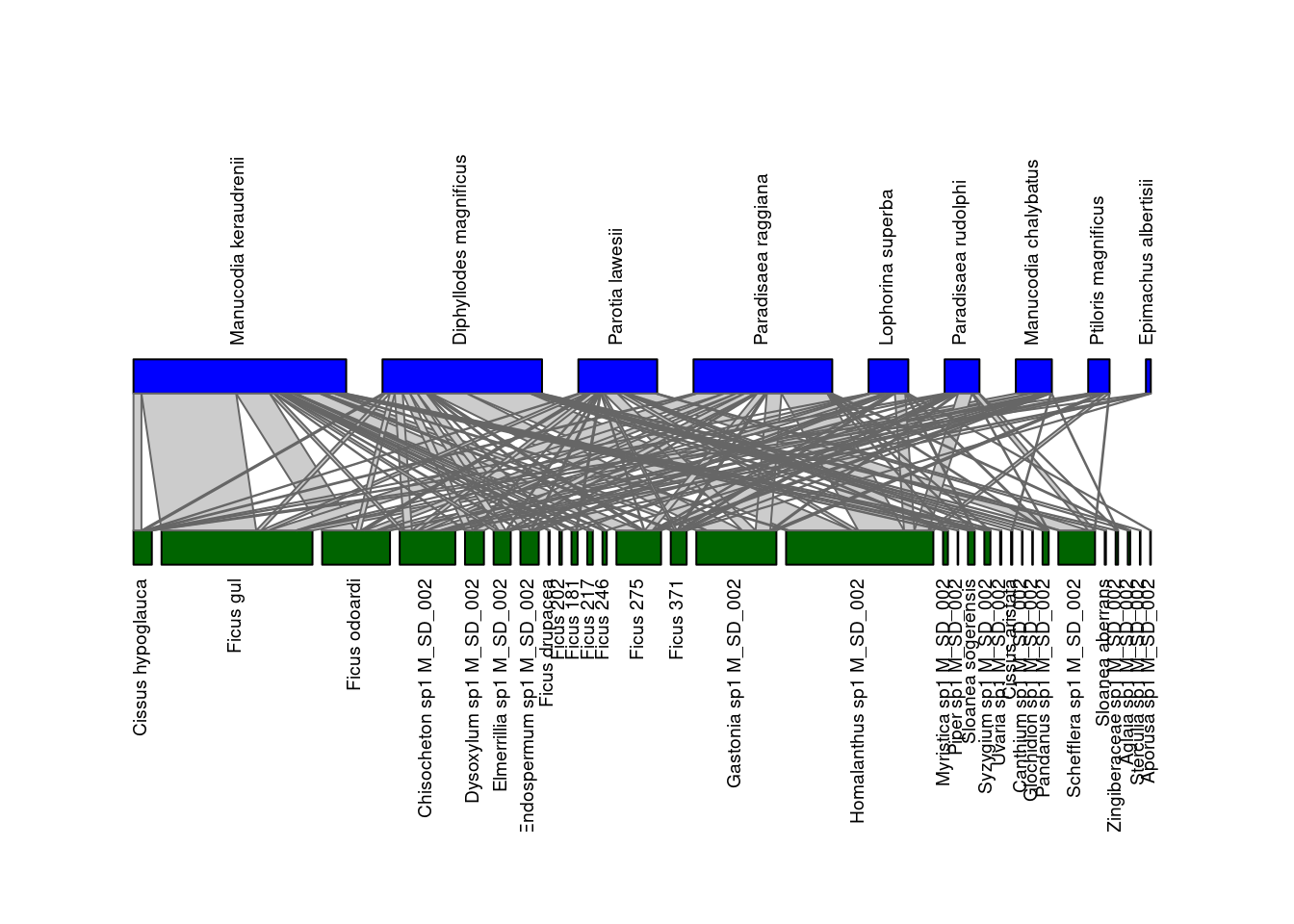

1.2.5 Exercise 2

From Web of life choose one foodweb on in the subset FW_017, download it, convert it into an adjacency matrix, and visualize it using igraph, using at least two layouts.
How is cannibalism displayed in the plot of a directed graphs representing a foodweb?
Is the adjacency matrix corresponding to a foodwed symmetric?
Def.: Symmetric is a matrix \(A\) for which \(A_{ij}=A_{ji}\).
Download the pollination network M_PL_024 from Web of life, convert it into an incidence matrix, and visualize it using bipartite.
SAVE YOUR DATA: It is important that you save the data needed for a plot or analysis so that instructors can reproduce your output without running the whole script again. For this specific assignment, this can be done running the following command

save(FW_017_03_graph, adj_matrix, 
     M_PL_024_graph, inc_matrix,
     file="~/ecological_networks_2024/workspace/03-14_toolkit_network_analysis/data_ex2.RData")

CHECK: The *RData file should appear in the folder 03-14_toolkit_network_analysis. If you want to be hundred percent sure that everything worked well, you can reload the variables from the created file:

load("~/ecological_networks_2024/workspace/03-14_toolkit_network_analysis/data_ex2.RData")

and produce your plots again.

1.3 Connectance of pollination networks

The connectance is one of the properties characterizing a network and is defined as the ratio between the actual number of links (i.e. pairwise interactions among species) and the maximal number of links that could be realized in that type of network. For a bipartite network at most all the species of one group (e.g. plants) can interact with all the species of the other group (e.g. animals). Let us focus on pollination networks for which the connectance is defined as \[\begin{equation} \frac{\# \, links}{(\# \, plants) \times (\# animals)} \,. \end{equation}\] (The definition of connectance for a foodweb will be discussed in the questions and in forthcoming lectures).

1.3.1 Compute the connectance from an edge list

Our goal is to compute the connectance for all the pollination networks available on Web of life and store its value in a dataframe along with the size of the incidence matrix associated with each network.
We start downloading all the networks with interaction_type=Pollination

json_url <- paste0(base_url,"get_networks.php?interaction_type=Pollination") 
pol_nws <- jsonlite::fromJSON(json_url)
class(pol_nws$connection_strength) <-"numeric"
head(pol_nws)

##   network_name             species1              species2 connection_strength
## 1     M_PL_063       Lantana camara  Phaethornis eurynome                   1
## 2     M_PL_063       Lantana camara   Stephanoxis lalandi                  26
## 3     M_PL_063        Fuchsia regia  Phaethornis eurynome                   6
## 4     M_PL_063        Fuchsia regia  Thalurania glaucopis                   5
## 5     M_PL_063        Fuchsia regia Clytolaema rubricauda                  15
## 6     M_PL_063 Psychotria leiocarpa  Thalurania glaucopis                   2

When data, for a given network, is given in the form of edge list, computing the connectance is straightforward: one just needs to count the number of rows in the data frame (links) and the distinct rows in the column species1 (e.g. plants) and species2 (e.g. animals).
We first create a dataframe containing only the distinct network names

pol_nw_names <- distinct(pol_nws, network_name)

Now we perform a for loop on the network names and compute the connectance and the size of the relative incidence matrix

# initialize dataframe  to store results 
pol_connectance_df <- NULL         

for (nw_name in pol_nw_names$network_name){
  
  nw <- filter(pol_nws, network_name == nw_name) 
  
  links <- nw %>% nrow() 
  plants <- distinct(nw, species2) %>%  nrow() 
  animals <- distinct(nw, species1) %>% nrow()
  size <- plants*animals
  conn <- links/size    
  
  conn_row <- data.frame(nw_name, size, conn)
  
  pol_connectance_df <- rbind(pol_connectance_df, conn_row)
}

colnames(pol_connectance_df) <- c("network_name", "size", "connectance")

You can visualize the results as usual:

pol_connectance_df %>% head() %>% formattable()

network_name	size	connectance
M_PL_063	495	0.2484848
M_PL_064	112	0.2857143
M_PL_065	105	0.4190476
M_PL_066	155	0.4709677
M_PL_067	155	0.3806452
M_PL_068	279	0.2974910

# remove %>% head() to see the whole dataframe

ACHTUNG: The Web of life API returns a dataframe in which only meaningful values for the connection_strength are given. Generally, it will be wise to check if all interaction values are non-vanishing and possibly filter out from the edge list the rows corresponding to vanishing or NA connection_strength. In pseudo code, this is done as follows

pol_nws_good <- filter(pol_nws, connection_strength > 0) %>% 
  filter(., !is.na(connection_strength))

The next plot shows the connectance of all pollination networks versus the incidence-matrix size for each network:

# import the ggplot2 package (if not done at the beginning) 
library(ggplot2)

# define a function to plot as guide to the eye
guide_eye <- function(x,c,alpha){
  return(c/x**alpha)
}


options(repr.plot.width=5, repr.plot.height=4)
ggplot() +
  ggtitle("Pollination networks") +
  stat_function(fun = function(x) guide_eye(x,4.8,0.5), color ="black", linetype = "dotted") +
  geom_point(data = pol_connectance_df, aes(size, connectance), color = "purple", shape=1) +
  labs(x = "Incidence matrix size", 
       y = "Network connectance") +
  scale_x_continuous(trans='log10') +
  scale_y_continuous(trans='log10')

1.3.2 Filter by latitude

Now we would like to display with a different color the connectance of the subset of networks in the tropical area. We start downloading the metadata of all networks in Web of life (see above)

nws_info <- read.csv(paste0(base_url,"get_network_info.php")) 
my_nws_info <- select(nws_info, network_name, location, latitude,longitude)

From this dataframe we select the names of networks recorded in the tropical region, namely in the area with latitude between -23.43647\(^\circ\) and 23.43647\(^\circ\).

tropical_nws_info <- nws_info %>% filter(.,between(latitude, -23.43647, 23.43647))  
tropical_nw_names <- distinct(tropical_nws_info, network_name)

Now we keep in the dataframe pol_connectance_df only the data corresponding to tropical networks. In practice, we look for the intersection of the two ensembles: polination networks and tropical networks

tropical_pol_conn_df <- filter(pol_connectance_df, network_name %in% tropical_nw_names$network_name) %>%
  select(network_name, size, connectance)

At this point we can superimpose the (orange) points calculated for tropical networks to the previous plot

options(repr.plot.width=5, repr.plot.height=4)
ggplot() +
  ggtitle("Tropical pollination networks") +
  stat_function(fun = function(x) guide_eye(x,4.,0.5), color ="black", linetype = "dotted") +
  geom_point(data = pol_connectance_df, aes(size, connectance), color = "purple", shape=1) +
  geom_point(data = tropical_pol_conn_df, aes(size, connectance), color = "dark orange") +
  labs(x = "Incidence matrix size", 
       y = "Network connectance") +
  scale_x_continuous(trans='log10') +
  scale_y_continuous(trans='log10')

1.3.3 Exercise 3

Given that a food-web is typically represented by a square (adjacency) matrix, what would be in your opinion a sound definition of connectance in that case?
(Hint think of the maximal number of possible links and normalize accordingly)
What is the functional dependence of the black line plotted on top of the graphs (note the scales are log-log)?
Superimpose the connectance computed for few selected networks at your choice to the previous plot and comment your observation.
(Hint insert the selected network names in the script provided below)

# put the selected network names in this vector as strings
my_nw_names <-  c( )

my_pol_conn_df <- filter(pol_connectance_df, network_name %in% my_nw_names) %>%
  select(network_name, size, connectance)

options(repr.plot.width=5, repr.plot.height=4)
ggplot() +
  ggtitle("My pollination networks") +
  stat_function(fun = function(x) guide_eye(x,4.,0.5), color ="black", linetype = "dotted") +
  geom_point(data = pol_connectance_df, aes(size, connectance), color = "purple", shape=1) +
  geom_point(data = my_pol_conn_df, aes(size, connectance), color = "black") +
#  geom_point(data = tropical_pol_conn_df, aes(size, connectance), color = "dark orange") +
  labs(x = "Incidence matrix size", 
       y = "Network connectance") +
  scale_x_continuous(trans='log10') +
  scale_y_continuous(trans='log10')

SAVE YOUR DATA: For this specific assignment, this can be save the relevant variables running the following command

save(pol_connectance_df, tropical_pol_conn_df, my_pol_conn_df, 
     file="~/ecological_networks_2024/workspace/03-14_toolkit_network_analysis/data_ex3.RData")

CHECK: Another *RData file should appear in the folder 03-14_toolkit_network_analysis. If you want to be hundred percent sure that everything worked well, you can reload the variables from the created file:

load("~/ecological_networks_2024/workspace/03-14_toolkit_network_analysis/data_ex3.RData")

and produce your plots again.

Solutions

Exercise 1

\(\bullet\) How many networks are stored in the Web of life database? how many pollination and seed-dispersal networks?

\(\bullet\) How many entries in the M_PL_073 network are not taxonomically resolved down to the species level?

\(\bullet\) How many networks in Web of life have been collected in the tropical region?

ANSWER:
The questions above are addressed point by point running the underlying lines of code:

json_url <- paste0(base_url,"get_networks.php") 
all_nws <- jsonlite::fromJSON(json_url)# extract all nws
all_nw_names <- distinct(all_nws, network_name) # unique nw names extracted

no_unique_networks <- length(all_nw_names$network_name) # get the length of the vector
no_unique_networks                                      # with all the unique networks (names)
# There are 319 networks stored on the Web of Life database

# get all distinct pollination networks
json_url <- paste0(base_url,"get_networks.php?interaction_type=Pollination") 
pol_nws <- jsonlite::fromJSON(json_url)
pol_nw_names <- distinct(pol_nws, network_name)
no_pollination_networks <- nrow(pol_nw_names)
no_pollination_networks
# There are 172 pollination networks stored on the Web of Life database

all_nw_info <- read.csv(paste0(base_url,"get_network_info.php"))
my_nw_info <- select(all_nw_info, network_name, location, latitude, longitude, region)
sd_nws <- all_nw_info %>%
  filter(network_type == "Seed Dispersal")
sd_nw_names <- distinct(sd_nws, network_name)
no_sd_networks <- nrow(sd_nw_names)
no_sd_networks
# There are 34 seed-dispersal networks stored on the Web of Life database

# define the full url associated with the endpoint that downloads the M_PL_073 network
json_url <- paste0(base_url,"get_networks.php?network_name=M_PL_073")

# get dataframe
M_PL_073_nw <- jsonlite::fromJSON(json_url)

# download species info dataframe of the M_PL_073 network
M_PL_073_info <- read.csv(paste0(base_url,"get_species_info.php?network_name=M_PL_073"))

# filter for taxonomic.resolution not Species
M_PL_073_info_filtered <- filter(M_PL_073_info, taxonomic.resolution != "Species")

# length of this dataframe = number of entries with Taxonomic Resolution not down to Species level
nrow(M_PL_073_info_filtered)
# There are 4 entries in the M_PL_073 network that are not taxonomically resolved down to the species level

tropical_nws_info <- all_nw_info %>%
  filter(.,between(latitude, -23.43647, 23.43647))

no_tropica_nws <- nrow(tropical_nws_info)
no_tropica_nws
# there are 151 networks in WoL database that were collected in the tropics

Exercise 2

\(\bullet\) From Web of life choose one foodweb on in the subset FW_017, download it, convert it into an adjacency matrix, and visualize it using igraph, using at least two layouts.

ANSWER:
Repeat the same procedure described for the foodweb FW_002 in the example, working with the adjacency matrix.

\(\bullet\) How is cannibalism displayed in the plot of a directed graphs representing a foodweb?

ANSWER:
When cannibalism occurs within a species, a self-loop appear, in the graphical representation of that node in the network, namely a directed link points back to the node from where it originats.

\(\bullet\) Is the adjacency matrix corresponding to a foodwed symmetric?
Def.: Symmetric is a matrix \(A\) for which \(A_{ij}=A_{ji}\).

ANSWER:
No, \(A_{ij}=A_{ji}\) would mean that every predator is also predated by its prey. So the adjaciency matrix is not symmetric in general. When links represent an interaction, like in pollination or seed-dispersal networks, then \(A_{ij}=A_{ji}\). In those cases, the whole information is already contained in the incidence matrix.

\(\bullet\) Download the pollination network M_PL_024 from Web of life, convert it into an incidence matrix, and visualize it using bipartite.

ANSWER:
Repeat the same procedure described for the seed-dispersal network M_SD_002 in the example, working with the incidence matrix, after having performed the bipartite mapping.

Exercise 3

\(\bullet\) Given that a food-web is typically represented by a square (adjacency) matrix, what would be in your opinion a sound definition of connectance in that case?

ANSWER:
The maximal number of links that could be realized in a foodweb is given by the number of elements in the upper (or the lower) triangle of the adjaciency matrix \[\begin{equation} \frac{N (N +1)}{2} \, , \end{equation}\] \(N\) being the number of raws and columns of the adjaciency matrix itself, therefore the connectance is defined as follows: \[\begin{equation} \frac{2 \# \, links}{N} \,. \end{equation}\]

\(\bullet\) What is the functional dependence of the black line plotted on top of the graphs (note the scales are log-log)?

ANSWER:
It is a power law \[\begin{equation} y = C x^{-\gamma} \end{equation}\] with \(\gamma=0.5\), in the present case.

\(\bullet\) Superimpose the connectance computed for few selected networks at your choice to the previous plot and comment your observation.

ANSWER:
You need to fill the vector my_nw_names with some networks names such as

my_nw_names <- c("M_PL_063", "M_PL_061_11", "M_PL_036")
#...

and comment on how the connectance of the chosen networks compares with the guide to the eye and other netowrks of similar size. An alternative could have been to filter a group of networks by latitude of longitude or by region (e.g. Europe).