5 Null models
Fernando Pedraza
session 21/03/2024
5.1 Null models by hand
In this section you will randomize networks “by hand” following some of the null models covered during the morning lecture. Some null models will require you to generate random numbers and perform simple arithmetic operations. Use R for these purposes (hint: use the runif() function to generate random numbers).
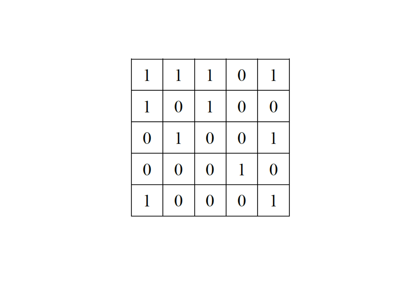
1. Consider a network represented by the following adjacency matrix:

Provide a randomization of the matrix using:
A. The Equifrequent Null Model
Copy the matrix to your Rscript file, replace the ’x’s with the zeros or ones resulting from the randomization.
# -----------------------------------------------------------
#|           |           |           |           |           |
#|     x     |     x     |     x     |     x     |     x     |
#|           |           |           |           |           |
#|-----------------------------------------------------------|
#|           |           |           |           |           |
#|     x     |     x     |     x     |     x     |     x     |
#|           |           |           |           |           |
#|-----------------------------------------------------------|
#|           |           |           |           |           |
#|     x     |     x     |     x     |     x     |     x     |
#|           |           |           |           |           |
#|-----------------------------------------------------------|
#|           |           |           |           |           |
#|     x     |     x     |     x     |     x     |     x     |
#|           |           |           |           |           |
#|-----------------------------------------------------------|
#|           |           |           |           |           |
#|     x     |     x     |     x     |     x     |     x     |
#|           |           |           |           |           |
# -----------------------------------------------------------
B. The Probabilistic Cell Null Model
Copy the matrix to your Rscript file, replace the ’x’s with the zeros or ones resulting from the randomization.
# -----------------------------------------------------------
#|           |           |           |           |           |
#|     x     |     x     |     x     |     x     |     x     |
#|           |           |           |           |           |
#|-----------------------------------------------------------|
#|           |           |           |           |           |
#|     x     |     x     |     x     |     x     |     x     |
#|           |           |           |           |           |
#|-----------------------------------------------------------|
#|           |           |           |           |           |
#|     x     |     x     |     x     |     x     |     x     |
#|           |           |           |           |           |
#|-----------------------------------------------------------|
#|           |           |           |           |           |
#|     x     |     x     |     x     |     x     |     x     |
#|           |           |           |           |           |
#|-----------------------------------------------------------|
#|           |           |           |           |           |
#|     x     |     x     |     x     |     x     |     x     |
#|           |           |           |           |           |
# -----------------------------------------------------------
2. Consider a network represented by the following adjacency matrix:
Provide three iterations of the swap null model:
Swap null model: first iteration
Copy the matrix to your Rscript file, replace the ’x’s with the zeros or ones resulting from the randomization.
# -----------------------------------------------------------
#|           |           |           |           |           |
#|     x     |     x     |     x     |     x     |     x     |
#|           |           |           |           |           |
#|-----------------------------------------------------------|
#|           |           |           |           |           |
#|     x     |     x     |     x     |     x     |     x     |
#|           |           |           |           |           |
#|-----------------------------------------------------------|
#|           |           |           |           |           |
#|     x     |     x     |     x     |     x     |     x     |
#|           |           |           |           |           |
#|-----------------------------------------------------------|
#|           |           |           |           |           |
#|     x     |     x     |     x     |     x     |     x     |
#|           |           |           |           |           |
#|-----------------------------------------------------------|
#|           |           |           |           |           |
#|     x     |     x     |     x     |     x     |     x     |
#|           |           |           |           |           |
# -----------------------------------------------------------
Swap null model: second iteration
Copy the matrix to your Rscript file, replace the ’x’s with the zeros or ones resulting from the randomization.
# -----------------------------------------------------------
#|           |           |           |           |           |
#|     x     |     x     |     x     |     x     |     x     |
#|           |           |           |           |           |
#|-----------------------------------------------------------|
#|           |           |           |           |           |
#|     x     |     x     |     x     |     x     |     x     |
#|           |           |           |           |           |
#|-----------------------------------------------------------|
#|           |           |           |           |           |
#|     x     |     x     |     x     |     x     |     x     |
#|           |           |           |           |           |
#|-----------------------------------------------------------|
#|           |           |           |           |           |
#|     x     |     x     |     x     |     x     |     x     |
#|           |           |           |           |           |
#|-----------------------------------------------------------|
#|           |           |           |           |           |
#|     x     |     x     |     x     |     x     |     x     |
#|           |           |           |           |           |
# -----------------------------------------------------------
Swap null model: third iteration
Copy the matrix to your Rscript file, replace the ’x’s with the zeros or ones resulting from the randomization.
# -----------------------------------------------------------
#|           |           |           |           |           |
#|     x     |     x     |     x     |     x     |     x     |
#|           |           |           |           |           |
#|-----------------------------------------------------------|
#|           |           |           |           |           |
#|     x     |     x     |     x     |     x     |     x     |
#|           |           |           |           |           |
#|-----------------------------------------------------------|
#|           |           |           |           |           |
#|     x     |     x     |     x     |     x     |     x     |
#|           |           |           |           |           |
#|-----------------------------------------------------------|
#|           |           |           |           |           |
#|     x     |     x     |     x     |     x     |     x     |
#|           |           |           |           |           |
#|-----------------------------------------------------------|
#|           |           |           |           |           |
#|     x     |     x     |     x     |     x     |     x     |
#|           |           |           |           |           |
# -----------------------------------------------------------
5.2 Computer part I
In this section we will use R code to run the null models covered during this morning’s lecture. We will focus on using the null models to evaluate the nestedness value of a single network. Ultimately, we want to know if the measured nestedness value of our network is significantly different from the nestedness values obtained from a set of random iterations. To do this, we will first define a network and compute its nestedness. Then, we’ll compute nestedness again using three null models. Finally, we will estimate the significance of nestedness using the z-score.
Before we begin we should load the packages we will use for this session. Please note that we will use the rweboflife package to run the null models and compute nestedness.
# Load packages
library(igraph)
library(tidyverse)
library(bipartite)

# To install the rweboflife package, uncomment the following line and run it:
#devtools::install_github("bascompte-lab/rweboflife", force = TRUE)

# Load rweboflife package
library(rweboflife)
5.2.1 Defining a network
For demonstration purposes, we will be using a perfectly nested network (10 rows x 10 columns) in this first part of the exercise. We begin by defining the network (stored as nested_mat) and visualising it.
# this function helps you to construct a perfectly nested matrix.
# as a arguments, you should specify the number of columns and rows.

perfect_nested <- function(my_cols, my_rows){

  mat <- matrix(0, my_rows, my_cols)

  for (i in seq(1,my_rows,1)) {
    j_max <- ceiling(i*my_cols/my_rows)

    for (j in seq(1,j_max,1)) {
      mat[i,j] <-1
    }
  }
  return(t(mat))
}

# create a perfectly nested 10 x 10 matrix
nested_mat <- perfect_nested(10, 10)

# plot the matrix
visweb(nested_mat)
5.2.2 The nestedness function
Now that we have defined our network, we measure its nestedness. We will calculate nestedness using the function nestedness from the rweboflife package.
 nestedness <- function(M){

      # this code computes the nestedness of a given incident matrix M
      # according to the definition given in
      # Fortuna, M.A., et al.: Coevolutionary dynamics shape the structure of
      # bacteria‐phage infection networks. Evolution 1001-1011 (2019).
      # DOI 10.1111/evo.13731

      # Make sure we are working with a matrix
      M <- as.matrix(M)
      # Binarize the matrix
      B <- as.matrix((M>0))
      class(B) <- "numeric"

      # Get number of rows and columns
      nrows <- nrow(B)
      ncols <- ncol(B)

      # Compute nestedness of rows
      nestedness_rows <- 0
      for(i in 1:(nrows-1)){
        for(j in (i+1): nrows){

          c_ij <- sum(B[i,] * B[j,])      # Number of interactions shared by i and j
          k_i <- sum(B[i,])               # Degree of node i
          k_j <- sum(B[j,])               # Degree of node j

          if (k_i == 0 || k_j==0) {next}  # Handle case if a node is disconnected

          o_ij <- c_ij / min(k_i, k_j)    # Overlap between i and j

          nestedness_rows <- nestedness_rows + o_ij
        }
      }

      # Compute nestedness of columns
      nestedness_cols <- 0
      for(i in 1: (ncols-1)){
        for(j in (i+1): ncols){

          c_ij <- sum(B[,i] * B[,j])      # Number of interactions shared by i and j
          k_i <- sum(B[,i])               # Degree of node i
          k_j <- sum(B[,j])               # Degree of node j
          if (k_i == 0 || k_j==0) {next}  # Handle case if a node is disconnected.

          o_ij <- c_ij / min(k_i, k_j)    # Overlap between i and j

          nestedness_cols <- nestedness_cols + o_ij
        }
      }

      # Compute nestedness of the network
      nestedness_val <- (nestedness_rows + nestedness_cols) / ((nrows * (nrows - 1) / 2) +
                        (ncols * (ncols - 1) / 2))

      return(nestedness_val)
    }
5.2.3 Computing nestedness
Let’s compute the nestedness value for the network we defined before, as in previous sessions.
# Calculate the nestedness value for our network and store it
nestedness_perfectly_nested <- rweboflife::nestedness(nested_mat)
nestedness_perfectly_nested
## [1] 1Next, we will implement the null models.
5.2.4 Equifrequent null model
First, we’ll start with the equifrequent null model. We can code the equifrequent model like this:
equifrequent_model <- function(M_in, iter_max){

      rows <- nrow(M_in)
      columns <- ncol(M_in)
      number_ones <- count_nonzero(M_in)
      count_ones <- 0

      M_equif <- matrix(0, rows, columns)

      while (count_ones < number_ones) {

        x <- ceiling(runif(1, min = 0, max = rows))
        y <- ceiling(runif(1, min = 0, max = columns))

        while (M_equif[x,y] == 1) {

          x <- ceiling(runif(1, min = 0, max = rows))
          y <- ceiling(runif(1, min = 0, max = columns))

        }

        M_equif[x,y] <- 1
        count_ones <- count_ones + 1;
      }

      return(M_equif)
    }
However, to run the equifrequent model, we will use the null_model function from the rweboflife package. This function takes three arguments:
M_inspecifies the matrix you wish to randomisemodelspecifies the null model you wish to use to randomise the matrix (you can choose from: “equifrequent”, “cell” and “swap”)iter_maxdetermines how many iterations to run. Note that this parameter is only relevant when running the swap algorithm.
To run the equifrequent model on the network we previously defined, we run the following command:
randomistion_equifrequent <-  rweboflife::null_model(M_in = nested_mat,
                                                        model = "equifrequent",
                                                        iter_max = 1)
Now that we have randomised the matrix, we can compute the nestedness of this randomisation.
# Calculate the nestedness value for our network and store it
nestedness_randomistion_equifrequent <- rweboflife::nestedness(
                                            randomistion_equifrequent)
nestedness_randomistion_equifrequent
## [1] 0.6448942The raw nestedness value differs between the empirical network and its randomisation. However, one single randomisation is not enough to draw a conclusion. Instead, we should perform several randomistations and compute the nestedness value of each one. Then, we can compare the nestedness value of the empirical networks with the distribution of nestedness values from our randomisations. Let’s generate 100 randomisations of our network and compute nestedness for each one.
# define number of randomisations
n <- 100

# run randomistations
nestedness_from_equifrequent <- replicate(n,  rweboflife::nestedness(
  rweboflife::null_model(M_in = nested_mat, model = "equifrequent",
                        iter_max = 1)), simplify=TRUE)
Now that we have our nestedness estimates, we need to estimate the significance of the nested value we initially observed using the z-score. The formula to estimate z-scores is:
\[ z-score = \frac{observed\ nestedness - mean(nestedness)}{sd(nestedness)} \]
To calculate the z-score, we first have to obtain the mean and the standard deviation of the nestedness values we obtain from our null model. The mean and standard deviation are calculated in R with the mean and sd functions, respectively. Run the command below in your Rscript file, make sure to add the required parameter values.
# Compute mean for nestedness values estimated by null model
mean_nestedness <- mean()
# Compute sd for nestedness values estimated by null model
sd_nestedness <- sd()
Now we can calculate the z-score for the null model. Run the command below in your Rscript file, make sure to add the required parameter values.
Finally we can calculate the probability associated to the z-score using the pnorm and setting the lower.tail parameter to FALSE. Run the command below in your Rscript file, make sure to add the required parameter values.
5.2.5 Probabilistic cell model
Now let’s move to the probabilistic cell model. We can code the probabilistic cell model like this:
    cell_model <- function(M_in, iter_max){

      rows <- nrow(M_in)
      columns <- ncol(M_in)

      # binarize M_in
      M <- as.matrix((M_in>0))
      class(M) <- "numeric"

      PR <- matrix(0, rows, 1)
      PC <- matrix(0, columns, 1)
      M_cell <- matrix(0, rows, columns)

      for (i in 1:rows){
        number_ones <- 0
        for (j in 1:columns){
          if(M[i,j] == 1){
            number_ones <- number_ones + 1
          }
        }
        PR[i] <- number_ones/columns
      }

      for (j in 1:columns){
        number_ones <- 0
        for (i in 1:rows){
          if(M[i,j] == 1){
            number_ones <- number_ones + 1
          }
        }
        PC[j] <- number_ones/rows
      }

      for (i in 1:rows){
        for (j in 1:columns){
          p <- (PR[i]+PC[j])/2;
          r <- runif(1)
          if( r < p ){
            M_cell[i,j] <- 1;
          }
        }

      }

      return(M_cell)
    }
Repeat the same process we followed for the equifrequent null model, but now using the probabilistic cell model. You should do the following:
- Run the null model 100 times using the
null_modelfunction. - Compute the mean and standard deviation of our null model estimates.
- Calculate the z-score.
- Obtain an associated p-value.
5.2.6 Swap model
Lastly, we focus on the swap model. We can code the swap model like this:
    swap_model = function(M_in, iter_max){

      nr <- nrow(M_in) # number of rows
      nc <- ncol(M_in) # number of columns

      # initialize M (randomized matrix) iter loop
      M <- M_in

      for(iter in 1:iter_max){

        # binarize M into a logical matrix
        B <- as.matrix((M>0))

        # flatten logical matrix with row-major order
        M_vec <- as.vector(t(B))

        allEqual <- TRUE
        while (allEqual == TRUE){
          indexes <- create_indexes(nr, nc)
          sub_vec <- M_vec[indexes]
          allEqual <- xor(all(sub_vec), all(!(sub_vec)))
        }

        # shaffle indexes till all positions are swapped
        fullRND <- FALSE
        while (fullRND == FALSE){
          indexes_rnd <- indexes[shuffle(indexes)]
          fullRND <- all(indexes_rnd != indexes)
        }

        M_vec[indexes_rnd] <- sub_vec
        M_swap <- matrix(M_vec, nrow=nr, ncol=nc, byrow=TRUE) # back to matrix

        M <- M_swap
        class(M_swap) <- "numeric"
      }

      return(M_swap)
    }
Repeat the same process we followed for the other two null models, but now using the swap model. You should do the following:
- Run the null model 100 times with using the
null_modelfunction. Note that this time you should use theiter_maxparameter to specify that the null model should perform 1000 iterations.
- Compute the mean and standard deviation of our null model estimates.
- Calculate the z-score.
- Obtain an associated p-value.
5.3 Computer part II
In this final section we will use null models to test whether a set of pollination networks are significantly more or less nested than a set of seed dispersal networks.
5.3.1 Code
To save some time, I have already downloaded the necessary networks. The first thing we need to is to load the networks. The seed dispersal networks are stored as entries in the list called seed_networks which is found in the seed_networks.Rdata file. The pollination networks are stored as entries in the list called pollination_networks which is found in the pollination_networks.Rdata file. We will begin by loading these two files.
# Load pollination networks
load("~/ecological_networks_2024/downloads/Data/null_models/pollination_networks.Rdata")

# Load seed networks
load("~/ecological_networks_2024/downloads/Data/null_models/seed_networks.Rdata")
Now that we have our networks, we can run the null models. For this exercise, we will use the cell null model. Let’s outline our workflow:
- First, compute the nestedness value of each of the networks in the
seed_networksandpollination_networkslists. - Next, perform 20 randomisations of each network using the cell null model.
- Finally, run a t-test to determine whether there are differences between the two types of networks in relation to their standardized nestedness values.
Below you will find the code to perform the workflow outlined above. However, if you’re up for a challenge, feel free to write your own code. Use the p-value you obtain to answer the question at the bottom of this exercise.
#################################################
# SEED DISPERSER NETWORKS
#################################################

# calculate nestedness value of empirical networks
seed_nestedness <- sapply(seed_networks,  rweboflife::nestedness)

# generate 20 randomisations of each seed dispersal network using the equifrequent model
seed_randomisations <- replicate(20, lapply(seed_networks,  rweboflife::null_model,
                                            model = 'cell' ))

# compute the nestedness value of each randomisation
seed_randomisations_nestedness <- sapply(seed_randomisations,  rweboflife::nestedness)

# extract nestedness value of each randomisation
seed_randomisations_nestedness <- split(seed_randomisations_nestedness,
                                        ceiling(seq_along(seed_randomisations_nestedness)/20))

# compute mean nestedness of each randomisation
mean_seed_randomisations_nestedness <- sapply(seed_randomisations_nestedness, mean)

# compute sd nestedness of each randomisation
sd_seed_randomisations_nestedness <- sapply(seed_randomisations_nestedness, sd)

# calculate z-score of each network
seed_z_score <- (seed_nestedness - mean_seed_randomisations_nestedness)/
                 sd_seed_randomisations_nestedness


#################################################
# POLLINATION NETWORKS
#################################################

# calculate nestedness value of empirical networks
pollination_nestedness <- sapply(pollination_networks,  rweboflife::nestedness)

# generate 20 randomisations of each seed dispersal network using the equifrequent model
pollination_randomisations <- replicate(20, lapply(pollination_networks,
                                                   rweboflife::null_model,
                                                   model = 'cell'))

# compute the nestedness value of each randomisation
pollination_randomisations_nestedness <- sapply(pollination_randomisations,
                                                rweboflife::nestedness)

# extract nestedness value of each randomisation
pollination_randomisations_nestedness <- split(pollination_randomisations_nestedness,
                                               ceiling(seq_along(pollination_randomisations_nestedness)/20))

# compute mean nestedness of each randomisation
mean_pollination_randomisations_nestedness <- sapply(pollination_randomisations_nestedness,
                                                     mean)

# compute sd nestedness of each randomisation
sd_pollination_randomisations_nestedness <- sapply(pollination_randomisations_nestedness,
                                                   sd)

# calculate z-score of each network
pollination_z_score <- (pollination_nestedness - mean_pollination_randomisations_nestedness)/
                        sd_pollination_randomisations_nestedness


#################################################
# COMPARE NETWORKS
#################################################

# Calculate t-test to compare vector of zscores
t.test(seed_z_score,pollination_z_score)
5.3.2 Question
Have a look at the output of the t-test. Are there differences in the nestedness of the networks? Why do you think we observe this result? How do your findings relate to the main finding described by Bascompte et al. 20031?
Solutions
# Solutions for Exercise 4: Null models
# Fernando Pedraza
# fernando.pedraza@ieu.uzh.ch

##### Null models by hand #####

# I will not provide a solution for the first section on performing the null
# models by hand as your randomisations will most likely differ from mine.

##### Computer part I #####

# load package
library(rweboflife)

# define function to construct perfectly nested network
perfect_nested <- function(my_cols, my_rows){

  mat <- matrix(0, my_rows, my_cols)

  for (i in seq(1,my_rows,1)) {
    j_max <- ceiling(i*my_cols/my_rows)

    # print(i)
    # print(j_max)
    # print("")

    for (j in seq(1,j_max,1)) {
      mat[i,j] <-1
    }
  }
  return(t(mat))
}


# create a perfectly nested 10 x 10 matrix
nested_mat <- perfect_nested(10, 10)

# Calculate the nestedness value for the perfectly nested network
nestedness_perfectly_nested <- rweboflife::nestedness(nested_mat)
nestedness_perfectly_nested


# EQUIFREQUENT NULL MODEL

# define number of randomisations
n <- 100

# run randomistations
nestedness_from_equifrequent <- replicate(n,  rweboflife::nestedness(
  rweboflife::null_model(M_in = nested_mat, model = "equifrequent",
                         iter_max = 1)), simplify=TRUE)

# Compute mean for nestedness values estimated by null model
mean_nestedness_from_equifrequent <- mean(nestedness_from_equifrequent)
# Compute sd for nestedness values estimated by null model
sd_nestedness_from_equifrequent <- sd(nestedness_from_equifrequent)
# Compute z score following the formula
z_equifrequent <-  (nestedness_perfectly_nested - mean_nestedness_from_equifrequent)/sd_nestedness_from_equifrequent
# Compute associated p value
p_val_equifrequent <-pnorm(z_equifrequent, lower.tail = FALSE)
# Print p value
print(p_val_equifrequent)

# PROBABILISTIC CELL MODEL

# define number of randomisations
n <- 100

# run randomistations
nestedness_from_cell <- replicate(n,  rweboflife::nestedness(
  rweboflife::null_model(M_in = nested_mat, model = "cell",
                         iter_max = 1)), simplify=TRUE)

# Compute mean for nestedness values estimated by null model
mean_nestedness_from_cell <- mean(nestedness_from_cell)
# Compute sd for nestedness values estimated by null model
sd_nestedness_from_cell <- sd(nestedness_from_cell)
# Compute z score following the formula
z_cell <-  (nestedness_perfectly_nested - mean_nestedness_from_cell)/sd_nestedness_from_cell
# Compute associated p value
p_val_cell <-pnorm(z_cell, lower.tail = FALSE)
# Print p value
print(p_val_cell)


# SWAP MODEL

# define number of randomisations
n <- 100

# run randomistations
nestedness_from_swap <- replicate(n,  rweboflife::nestedness(
  rweboflife::null_model(M_in = nested_mat, model = "swap",
                         iter_max = 1000)), simplify=TRUE)

# Compute mean for nestedness values estimated by null model
mean_nestedness_from_swap <- mean(nestedness_from_swap)
# Compute sd for nestedness values estimated by null model
sd_nestedness_from_swap <- sd(nestedness_from_swap)
# Compute z score following the formula
z_swap <-  (nestedness_perfectly_nested - mean_nestedness_from_swap)/sd_nestedness_from_swap
# Compute associated p value
p_val_swap <-pnorm(z_swap, lower.tail = FALSE)
# Print p value
print(p_val_swap)


# QUESTION

# Compare the conclusions about the significance of nestedness across the three null models.
# In your Rscript, discuss any differences you may have obtained.

print(p_val_equifrequent) # 3.056868e-35
print(p_val_cell) # 2.102551e-07
print(p_val_swap) # 3.452796e-25

# You should observe that the p-values for all null models are highly significant.
# Note that your calculated p-values are most likely different from mine, that is ok!
# All null models suggest that the nestedness value of the perfectly nested network
# is highly significant, in other words it is very unlikely to have arisen by
# chance. You can also observe differences between the p-values. All are highly
# signficant, but in this case the p-value from the cell model is the largest one.
# This may suggest that this null model is more conservative than the others.


##### Computer part II #####

# Load pollination networks
load("~/ecological_networks_2024/downloads/Data/null_models/pollination_networks.Rdata")

# Load seed networks
load("~/ecological_networks_2024/downloads/Data/null_models/seed_networks.Rdata")


#################################################
# SEED DISPERSER NETWORKS
#################################################

# calculate nestedness value of empirical networks
seed_nestedness <- sapply(seed_networks,  rweboflife::nestedness)

# generate 20 randomisations of each seed dispersal network using the equifrequent model
seed_randomisations <- replicate(20, lapply(seed_networks,  rweboflife::null_model,
                                            model = 'cell' ))

# compute the nestedness value of each randomisation
seed_randomisations_nestedness <- sapply(seed_randomisations,  rweboflife::nestedness)

# extract nestedness value of each randomisation
seed_randomisations_nestedness <- split(seed_randomisations_nestedness,
                                        ceiling(seq_along(seed_randomisations_nestedness)/20))

# compute mean nestedness of each randomisation
mean_seed_randomisations_nestedness <- sapply(seed_randomisations_nestedness, mean)

# compute sd nestedness of each randomisation
sd_seed_randomisations_nestedness <- sapply(seed_randomisations_nestedness, sd)

# calculate z-score of each network
seed_z_score <- (seed_nestedness - mean_seed_randomisations_nestedness)/
  sd_seed_randomisations_nestedness


#################################################
# POLLINATION NETWORKS
#################################################

# calculate nestedness value of empirical networks
pollination_nestedness <- sapply(pollination_networks,  rweboflife::nestedness)

# generate 20 randomisations of each seed dispersal network using the equifrequent model
pollination_randomisations <- replicate(20, lapply(pollination_networks,
                                                   rweboflife::null_model,
                                                   model = 'cell'))

# compute the nestedness value of each randomisation
pollination_randomisations_nestedness <- sapply(pollination_randomisations,
                                                rweboflife::nestedness)

# extract nestedness value of each randomisation
pollination_randomisations_nestedness <- split(pollination_randomisations_nestedness,
                                               ceiling(seq_along(pollination_randomisations_nestedness)/20))

# compute mean nestedness of each randomisation
mean_pollination_randomisations_nestedness <- sapply(pollination_randomisations_nestedness,
                                                     mean)

# compute sd nestedness of each randomisation
sd_pollination_randomisations_nestedness <- sapply(pollination_randomisations_nestedness,
                                                   sd)

# calculate z-score of each network
pollination_z_score <- (pollination_nestedness - mean_pollination_randomisations_nestedness)/
  sd_pollination_randomisations_nestedness


#################################################
# COMPARE NETWORKS
#################################################

# Calculate t-test to compare vector of zscores
t.test(seed_z_score,pollination_z_score)

##
##  Welch Two Sample t-test
##
## data:  seed_z_score and pollination_z_score
## t = -0.7027, df = 17.625, p-value = 0.4914
## alternative hypothesis: true difference in means is not equal to 0
## 95 percent confidence interval:
##  -1.4311341  0.7145558
## sample estimates:
## mean of x mean of y
## 0.6255704 0.9838595

# QUESTION
# Have a look at the output of the t-test. Are there differences in the nestedness of the networks?
# Why do you think we observe this result? How do your findings relate to the main finding
# described by Bascompte et al. 2003?

# From the t-test we can conclude that there are no significant differences in the nestedness values
# of pollination and seed dispersal networks (p = 0.49). This result is in agreement with the
# findings described in Bascompte et al. 2003.

# Why do you think we observe this result?
# Any reasonble hypothesis as to why this is the case (for example ecological or evolutionary
# mechanisms) is a valid answer.
Guimarães, P., Pires, M., Jordano, P. et al. Indirect effects drive coevolution in mutualistic networks. Nature 550, 511–514 (2017).↩︎