10 Models of evolution in networks
Leandro Cosmo
session 11/04/2024
10.1 About this session
In this session you will be implementing the coevolution model proposed in Guimaraes et al. 20172. This tutorial is split into 4 sections.
- A brief description of the coevolution model, its equations and some code to implement it in R.
- A demonstration of how to simulate the trait evolution of a pairwise interaction.
- An exercise where you will simulate the trait evolution of a small network.
- An exercise where you will simulate the trait evolution across networks with different structures.
The goal of this tutorial is for you to get an intuitive understanding of how the model works and what its predictions entail. You should gain an understanding of how changing the strength of mutualistic selection and the structure of a network shapes the coevolution of traits.
You will have to write some code to complete the exercises, but it will be mostly similar to the code I provide you in the demonstrations. If you find the code overwhelming I can walk you through it, feel free to ask questions during the exercise session or email me at leandro.giacobellicosmo@uzh.ch. If you’re up for a challenge, you can rewrite my code to make it more efficient.
10.2 Section 1: The coevolution model
We will be using the coevolutionary model proposed in Guimaraes et al 2017. As described during the lecture, the model incorporates coevolutionary dynamics and network structure to model trait evolution. The equation is the following:
\[ Z_i^{(t+1)} = Z_i^{(t)} + \phi_{i}\left[m_i \sum_{j,j\neq{i}}q_{ij}^{(t)}(Z_{j}^{(t)}-Z_{i}^{(t)}) + \left(1 - m_i\right)(\theta_{i}-Z_{i}^{(t)})\right]\]
where \(Z_i^{(t)}\) is the mean trait value of the local population of speices i at time t. \(\phi\) is a compound parameter that affects the slope of the selection gradient. N is the number of species in the network. \(q_{ij}^{(t)}\) is the interaction weight that describes the evolutionary effect of species j on the selection gradient of species i and evolves over time because of trait matching. \(\theta\) is the phenotype favoured by environmental selection. For more information on model parameters, refer to Guimaraes et al. 2017.
Note that:
\[ q_{ij}^{(t)} = \frac{a_{ij}e^{-\alpha(Z_{j}^{(t)}-Z_{i}^{(t)})^{2}}}{\sum_{k, i\neq{k}}^{N}a_{ik}e^{-\alpha(Z_{k}^{(t)}-Z_{i}^{(t)})^{2}}}\]
where \(m_i\) is the level of mutualistic selection and \(\alpha\) is a scaling constant that controls the sensitivity of the evolutionary effect to trait matching (this is set to 0.2 as in Guimaraes et al. 2017).
Given the model, we need to build a function in R that takes the required parameters and computes trait evolution. This the function that we will be using to run the model. Notice that the function coevolution_model also incorporates a parameter (epsilon) that determines whether the model has reached an equilibrium. The function also has a parameter (t_max) that sets the maximum number of time steps to simulate. Look over the function and try to link each line of code to operations in the model.
# Code for coevolutionary model
coevolution_model = function(f, m_value){
  # Function to model trait evolution in a mutualistic network

  # Arguments:
  # f: square adjacency matrix representing the mutualistic network
  # m: strength of mutualistic selection

  # Returns:
  # A data frame with the timesteps, trait values, species names, and theta values
  #
  # Set parameters that model will use
  #
  # Define the number of species
  n_sp = dim(f)[1]
  # Define alpha
  alpha = 0.2
  # Define the distribution for phi
  phi_mean = 0.7
  phi_sd = 0.01
  # Draw phi value for species
  set.seed(1)
  phi = rnorm(n_sp,phi_mean,phi_sd)
  # Define mutualism selection distribution
  m_mean = m_value
  m_sd = 0.01
  # Draw mutualism selection value for species
  set.seed(2)
  m = rnorm(n_sp,m_mean,m_sd)
  # Define range of theta values
  theta_min = 0
  theta_max = 10
  # Draw theta value for species
  set.seed(3)
  theta = runif(n_sp,min = theta_min,max = theta_max)
  # Draw initial trait value for species
  set.seed(4)
  init = runif(n_sp, min = theta_min, max = theta_max)
  # Define threshold to stop simulations
  epsilon = 0.000001
  # Define the max number of generations to simulate
  t_max = 10000


  # Initialize an empty matrix to store trait values.
  # The number of columns of the matrix is equal to the number of
  # species in the initial matrix
  # The number of rows of the matrix is equal to the maximum number of
  #simulation steps
  trait_sim_mat = matrix(NA,nrow=t_max,ncol=n_sp)
  colnames(trait_sim_mat) <- paste0('Species ', 1:n_sp)
  # Store initial trait values in first row of result matrix
  trait_sim_mat[1,] = init

  # Perform the simulation for a maximum of t_max-1 time steps
  for (time_step in 1:(t_max - 1)){
    # Define the trait values for the current simulation
    current_trait_values = trait_sim_mat[time_step,]
    # Compute the differences in trait values for all possible species
    # combinations
    # Results are stored as matrix
    trait_differences_mat = t(f*current_trait_values) - f*current_trait_values
    # Compute the q matrix
    # Values in this matrix represent the evolutionary effect that
    # species have on each other
    q = f*(exp(-alpha*(trait_differences_mat^2)))
    # Standardize the matrix to a maximum value of 1
    q_n = q / apply(q,1,sum)
    # Compute selection by mutualism
    q_m = q_n * m
    # Calculate selection differentials
    sel_dif = q_m * trait_differences_mat
    # Calculate trait change as a result of mutualism
    r_mut = phi * apply(sel_dif, 1, sum)
    # Calculate trait chagne as a result of environment
    r_env = phi * (1 - m)* (theta - current_trait_values)
    # Calculate trait change given mutualism and environment and update
    # matrix with results from simulation
    trait_sim_mat[time_step + 1,] = current_trait_values + r_mut + r_env # updating z values
    # Calculate how much trait changed from previous time step to
    # current one
    dif = mean(abs(current_trait_values - trait_sim_mat[time_step + 1,]))
    # If the the observed change in trait value is smaller than
    # epsilon, then exit loop
    if(dif < epsilon)
      break
  }

  # get the output
  matrix_output <- trait_sim_mat[1:(time_step+1),]
  # generate time steps
  time_step_vector <- rep(1:nrow(matrix_output), times = n_sp)
  # extract theta values
  theta_vector <- rep(theta, each = nrow(matrix_output))
  # convert to dataframe
  dataframe_output <- as.data.frame(matrix_output)
  # add column
  dataframe_output <- cbind(time_step_vector, melt(dataframe_output))
  # add the theta column
  dataframe_output$theta <- theta_vector
  # rename columns
  colnames(dataframe_output) <- c('time', 'species', 'trait_value', 'theta')
  # Return a matrix containing the evolution of traits
  return(dataframe_output)
}
After defining our function, lets run it under different scenarios.
10.3 Section 2: Running the coevolution on model on a pairwise interaction
Now we run coevolution_model with two interacting species. In this section we will run the simulation with progressively higher \(m\) values. We want to know how the strength of mutualistic selection alters the coevolution of traits.
Before we start, we load the packages we will be using for this exercise session:

10.3.2 Run simulations
First we define the adjacency matrix we will be using for the simulations.
Next we run the simulations with weak mutualistic selection
# Define the strength of mutualistic selection
weak_m <- 0.3
# Run simulations for weak m
coevolution_output_weak_m = coevolution_model(f,weak_m)
# Add the m value to our data frame
coevolution_output_weak_m$m <- weak_m
Now we move on to the scenario with intermediate mutualistic selection
# Define the strength of mutualistic selection
mid_m <- 0.6
# Run simulations for mid m
coevolution_output_mid_m = coevolution_model(f,mid_m)
# Add the m value to our data frame
coevolution_output_mid_m$m <- mid_m
Finally, we run the scenario with strong mutualistic selection
# Define the strength of mutualistic selection
strong_m <- 0.9
# Run simulations for strong m
coevolution_output_strong_m = coevolution_model(f,strong_m)
# Add the m value to our data frame
coevolution_output_strong_m$m <- strong_m
Next, we put all our results together and visualize them. In the plot I show how the trait value of each species changed through time. I show the environmental optimum of each species as dashed lines on the plot.
# Now we put all the results together
coevolution_output <- rbind(coevolution_output_weak_m,
                            coevolution_output_mid_m,
                            coevolution_output_strong_m)

# Plot result
ggplot(data = coevolution_output,aes(x=as.numeric(time),y=trait_value,col=species)) +
  geom_line() + geom_point(size=0.8) + theme_minimal() +
  geom_hline(aes(yintercept=theta, color = species),linetype="dashed") +
  xlab("Time") + ylab("Trait Value") + theme(legend.position = 'bottom') +
facet_grid(~m) 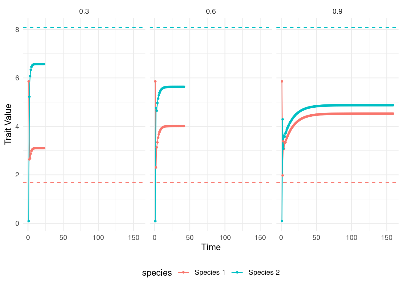
10.4 Section 3: Running the coevolution on model on a small network
Now you will run coevolution_model with four interacting species. Again, we will run the model with progressively stronger mutualistic selection. We want to know how the strength of mutualistic selection alters the coevolution of traits.

10.4.2 Your task
You will now simulate coevolution on the network shown above under three scenarios of mutualistic selection: 0.3, 0.6, and 0.9. You should produce a plot similar to the one we produced when simulating coevolution for two species.
# Work on your Rscript file to complete the task. You should do the following tasks:

# 1. Build the adjacency matrix
# 2. Simulate coevolution for the three different m values (remember to add the m value to your output!)
# 3. Combine the output from the three runs into a single dataframe
# 4. Plot the results
Once you’ve produced the plot, answer (write the answers in your Rscript) the following questions:
How does the strength of mutualistic selection affect the dynamics of trait evolution?
What differences can you observe in the trait evolution of species when going from a pairwise interactions to a (small) network?
10.5 Section 4: Simulating coevolution across networks with different structures
Now we are interested in exploring how network structure influences the outcome of coevolution of entire communities. To do this, we will simulate coevolution on a set of networks of identical size but with different connectance. I am providing you with these networks. Note that I have generated the networks artificially, by means of a model. Even though these are not empirical networks, they will allow us to explore our question of interest in this toy example.
First we load the networks.
# The networks are stored inside a list saved as an Rdata file.
load('~/ecological_networks_2024/downloads/Data/models_of_evolution_in_networks/list_of_networks.Rdata')
Next we define two new functions. The first is a slightly modified version of the coevolution model. This alternative version simulates coevolution on a given function and calculates the average trait matching between all species in the community. Larger values indicate higher trait similarity between species. This function also calculates the connectance of a network.
# Code for coevolutionary model
coevolution_model_across_networks = function(f, m_value){
  # Function to model trait evolution in a mutualistic network

  # Arguments:
  # f: square adjacency matrix representing the mutualistic network
  # m: strength of mutualistic selection

  # Returns:
  # A dataframe with the timesteps, trait values, species names, and theta values
  #
  # Set parameters that model will use
  #
  # convert incidence matrix to adjacency
  f <- as.matrix(as_adjacency_matrix(graph_from_incidence_matrix(as.matrix(f))))
  # Define the number of species
  n_sp = dim(f)[1]
  # Define alpha
  alpha = 0.2
  # Define the distribution for phi
  phi_mean = 0.7
  phi_sd = 0.01
  # Draw phi value for species
  set.seed(1)
  phi = rnorm(n_sp,phi_mean,phi_sd)
  # Define mutualism selection distribution
  m_mean = m_value
  m_sd = 0.01
  # Draw mutualism selection value for species
  set.seed(2)
  m = rnorm(n_sp,m_mean,m_sd)
  # Define range of theta values
  theta_min = 0
  theta_max = 10
  # Draw theta value for species
  set.seed(10)
  theta = runif(n_sp,min = theta_min,max = theta_max)
  # Draw initial trait value for species
  set.seed(11)
  init = runif(n_sp, min = theta_min, max = theta_max)
  # Define threshold to stop simulations
  epsilon = 0.000001
  # Define the max number of generations to simulate
  t_max = 10000

  # calculate the connectance of the current matrix
  network_connectance <- graph.density(graph_from_adjacency_matrix(f))

  # Initialize an empty matrix to store trait values.
  # The number of columns of the matrix is equal to the number of
  # species in the initial matrix
  # The number of rows of the matrix is equal to the maximum number of
  #simulation steps
  trait_sim_mat = matrix(NA,nrow=t_max,ncol=n_sp)
  colnames(trait_sim_mat) <- paste0('Species ', 1:n_sp)
  # Store initial trait values in first row of result matrix
  trait_sim_mat[1,] = init

  # Perform the simulation for a maximum of t_max-1 time steps
  for (time_step in 1:(t_max - 1)){
    # Define the trait values for the current simulation
    current_trait_values = trait_sim_mat[time_step,]
    # Compute the differences in trait values for all possible species
    # combinations
    # Results are stored as matrix
    trait_differences_mat = t(f*current_trait_values) - f*current_trait_values
    # Compute the q matrix
    # Values in this matrix represent the evolutionary effect that
    # species have on each other
    q = f*(exp(-alpha*(trait_differences_mat^2)))
    # Standardize the matrix to a maximum value of 1
    q_n = q / apply(q,1,sum)
    # Compute selection by mutualism
    q_m = q_n * m
    # Calculate selection differentials
    sel_dif = q_m * trait_differences_mat
    # Calculate trait change as a result of mutualism
    r_mut = phi * apply(sel_dif, 1, sum)
    # Calculate trait chagne as a result of environment
    r_env = phi * (1 - m)* (theta - current_trait_values)
    # Calculate trait change given mutualism and environment and update
    # matrix with results from simulation
    trait_sim_mat[time_step + 1,] = current_trait_values + r_mut + r_env # updating z values
    # Calculate how much trait changed from previous time step to
    # current one
    dif = mean(abs(current_trait_values - trait_sim_mat[time_step + 1,]))
    # If the the observed change in trait value is smaller than
    # epsilon, then exit loop
    if(dif < epsilon)
      break
  }

  # extract the trait values at equilibrium
  traits_at_equilibrium <- trait_sim_mat[time_step + 1,]
  # compute the degree of trait matching in the community
  matching_diff <- as.matrix(dist(traits_at_equilibrium,upper=TRUE,diag=TRUE))
  matching_at_equilibrium_all <- (exp(-alpha*((matching_diff)^2)))
  matching_at_equilibrium <- mean(rowMeans(matching_at_equilibrium_all,na.rm = TRUE))
  # return a vector with two elements:
  # The first is the connectance of the network.
  # The second is the euclidean distance of the traits in the community
  return(c(network_connectance,matching_at_equilibrium))
}
The second function allows us to run the coevolution model across all the networks in our list. As parameters, the function requires the list of networks we want to use and the strength of mutualistic selection we want the model to run. The function returns a vector with two elements. The first column contains the connectance values of each network. The second column contains the average trait matching in the community.
simulate_coevolution_across_networks <- function(list_of_networks, m_value){

  # create empty dataframe
  df <- NULL
  # loop through the list of networks
  for (i in 1:length(list_of_networks)) {
    # run the coevolution model for the current network with the specified mutualistic selection value
    current_coevolution_result <- coevolution_model_across_networks(list_of_networks[[i]], m_value = m_value)
    # append the results from the simulation to the dataframe
    df <- rbind(df, current_coevolution_result)
  }
  # make sure that the dataframe is in the correct format
  df <- as.data.frame(df)
  # rename the dataframe columns
  colnames(df) <- c('connectance', 'trait_matching')
  # return the dataframe
  return(df)

}
10.5.1 Your task
We are interested in seeing how connectance is related to the trait matching in a community after coevolution. Essentially, we want to know how network structure affects the similarity of traits in a community after they have coevolved. We also want to know if the relationship between network structure and trait matching changes as we increase the strength of mutualistic selection. To do this you will run simulate_coevolution_across_networks with list_of_networks twice, one with \(m = 0.1\) and the second with \(m = 0.9\).
After running the models you should produce two plots, one for \(m = 0.1\) and another for \(m = 0.9\). In both you should show the relationship between network connectance and trait matching. To help you to analyse the trend, fit a simple linear model to the plot (you can add a linear model to a ggplot using the following command: ggplot(...) + geom_smooth(method = 'lm')).
Once you have produced the plots, answer the following questions:
How does the connectance of a network relate to the similarity of traits in a community when coevolution is weak? What happens when coevolution is strong?
Can you come up with a hypothesis as to why we observe these patterns? What more simulations could you run to see if your hypothesis is true? (There is no wrong answer here, it’s perfectly fine to speculate!)
Guimarães, P., Pires, M., Jordano, P. et al. Indirect effects drive coevolution in mutualistic networks. Nature 550, 511–514 (2017).↩︎