4 Network-level metrics
Subhendu Bhandary and Alessandro Vindigni
session 20/03/2024
4.1 Nestedness
Nestedness is a measure of the structure of bipartite networks. Ecological networks, such as plant-pollinator networks, are often nested.
There there are many different measures of nestedness. We will focus on a modified version of the NODF measure (Almeida-Neto et al., 2008) which was used, for example, in Fortuna et al. (2019) to investigate networks of bacteria and phage. We recall the main concepts in these Slides.
The relevant literature is:
Almeida-Neto, M., Guimarães, P., Guimarães, P.R., Ulrich, W.: A consistent metric for nestedness analysis in ecological systems: reconciling concept and measurement. Oikos, 1227–1239 (2008). DOI 10.1111/j.2008.0030-1299.16644.xh
Fortuna, M.A., Barbour, M.A., Zaman, L., Hall, A.R., Buckling, A. and Bascompte, J.: Coevolutionary dynamics shape the structure of bacteria‐phage infection networks. Evolution 1001-1011 (2019). DOI 10.1111/evo.13731
4.1.1 Exercises (on paper)
This part of exercises is traditional and you are supposed to complete it on paper. Once you are done, please take a picture or scan your work (png, jpg, pdf, etc.) and upload it into the workspace of this sessions.
\(\bullet\) Write down the incidence matrix B and the degree of each node for the bipartite graph drawn below:

Hint: You can either solve this exercise on paper or use the following template to fill the matrix and copy it into your R script in the workspace.
$$
\\B = \begin{bmatrix}
0 & 0 & 0 & 0 & 0 & 0 \\
0 & 0 & 0 & 0 & 0 & 0 \\
0 & 0 & 0 & 0 & 0 & 0\\
0 & 0 & 0 & 0 & 0 & 0\\
\end{bmatrix}
$$
which is rendered in RMarkdown as \[ \\B = \begin{bmatrix} 0 & 0 & 0 & 0 & 0 & 0 \\ 0 & 0 & 0 & 0 & 0 & 0 \\ 0 & 0 & 0 & 0 & 0 & 0\\ 0 & 0 & 0 & 0 & 0 & 0\\ \end{bmatrix} \]
\(\bullet\) Compute on paper the nestedness of the bipartite graph defined by the incidence matrix \(B_2\).
\[ \\B_2 = \begin{bmatrix} 1 & 1 & 1 & 1 & 1 & 1 \\ 1 & 1 & 0 & 1 & 0 & 0 \\ 1 & 1 & 1 & 0 & 0 & 0 \\ 1 & 0 & 0 & 0 & 0 & 0 \\ 0 & 1 & 0 & 0 & 0 & 0 \\ \end{bmatrix} \]
\(\bullet\) Use R to check the result you obtained.
Hint: Use the following code to create the incidence matrix \(B_2\). Then, calculate its nestedness using the nestedness function of rweboflife package (see below).
4.2 Compute nestedness with rweboflife
The following code chunk downloads the network M_PL_026 from Web of life.
# Import the packages needed for this part
library(rjson)
library(dplyr)
library(rweboflife)
library(bipartite)
library(ggplot2)
library(latex2exp)
# define the base url
base_url <- "https://www.web-of-life.es/"
# Define the url associated with the network to be downloaded
json_url <- "https://www.web-of-life.es/get_networks.php?network_name=M_PL_026"
# Download the network (as a dataframe)
M_PL_026_nw <- jsonlite::fromJSON(json_url)

# Select the relevant columns and create the igraph object
M_PL_026_graph <- M_PL_026_nw %>%
  select(species1, species2, connection_strength) %>%
  graph_from_data_frame(directed=FALSE)
The following code chunk plots the network using functions from the bipartite package (uncomment the last lines if you prefer to use the igraph package).
# Convert the network into bipartite format
V(M_PL_026_graph)$type <- bipartite.mapping(M_PL_026_graph)$type
# Convert the igraph object into incidence matrix
M_PL_026_inc_mat <- as_incidence_matrix(M_PL_026_graph, attr="connection_strength", names=TRUE, sparse=FALSE)
# Convert elements into numeric values
class(M_PL_026_inc_mat) <- "numeric"
# Visualize the network with bipartite
plotweb(M_PL_026_inc_mat,
        method="normal", text.rot=90,
        bor.col.interaction="gray40",plot.axes=F, col.high="blue", labsize=1,
        col.low="darkgreen", y.lim=c(-1,3), low.lablength=40, high.lablength=40)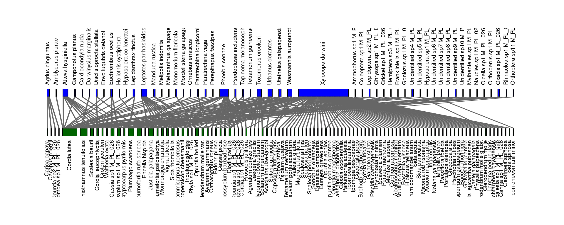
# Visualize the network with igraph (bipartite layout)
# plot(M_PL_026_graph,
#      layout=layout_as_bipartite,
#      arrow.mode=0,
#      vertex.label=NA,
#      vertex.size=4,
#      asp=0.2)
The degree distributions of this empirical network can be computed loading the function degree_distribution_df() from the helper.R file:
source("~/ecological_networks_2024/downloads/Functions/helper.R")
# create a dataframe with the degree distribution
M_PL_026_deg_dist <- degree_distribution_df(M_PL_026_graph)
library(formattable)
formattable(head(M_PL_026_deg_dist))| k | frequency |
|---|---|
| 0 | 0.00000000 |
| 1 | 0.66037736 |
| 2 | 0.15094340 |
| 3 | 0.06918239 |
| 4 | 0.01886792 |
| 5 | 0.02515723 |
annotation_1 <- data.frame(
  x = 15,
  y = 0.9,
  label = "empirical M_PL_026"
)

ggplot() +
  ggtitle("Degree distribution") +
  geom_point(data = M_PL_026_deg_dist, aes(k, frequency), shape = 16, color="black") +
  # Add text
  geom_text(data=annotation_1, aes( x=x, y=y, label=label),
            color="black",
            size=4 , angle=0) +
  # Add axes labels
  ylab(TeX("$P(k)$")) +
  xlab(TeX("$k$")) +
  coord_cartesian(xlim = c(0, 22), ylim = c(0.0001, 1.))
Now we would like to build a matrix that has the same size as the empirical pollination network M_PL_026 but is perfectly nested. To do this we can load the function perfect_nested() from the helper.R file:
source("~/ecological_networks_2024/downloads/Functions/helper.R")
nested_inc_mat <- perfect_nested(nrow(M_PL_026_inc_mat), ncol(M_PL_026_inc_mat))
You can check that the dimensions of the original and the nested matrix are the same
The nestedness function in the rweboflife package uses the Fortuna et al. (2019) nestedness measure. Below we load the nestedness function from the rweboflife package and check that the nestedness of the perfectly nested matrix actually equals 1:
# Import the rweboflife package
library(rweboflife)
# Compute network nestedness
rweboflife::nestedness(nested_inc_mat)
## [1] 1We can check that the matrix is actually perfectly nested by visual inspection. To do that it is convenient to color-code the matrix elements themselves. But first we have to order the columns:
# load package
library('plot.matrix')
nested_inc_mat_ordered <- nested_inc_mat[,order(colSums(nested_inc_mat),decreasing = TRUE)]

plot(nested_inc_mat_ordered, key=NULL, border=NA,  col.ticks=NA, # cex.axis=NA,
col=c('light grey','blue'), breaks=c(0, 0.5, 1)) 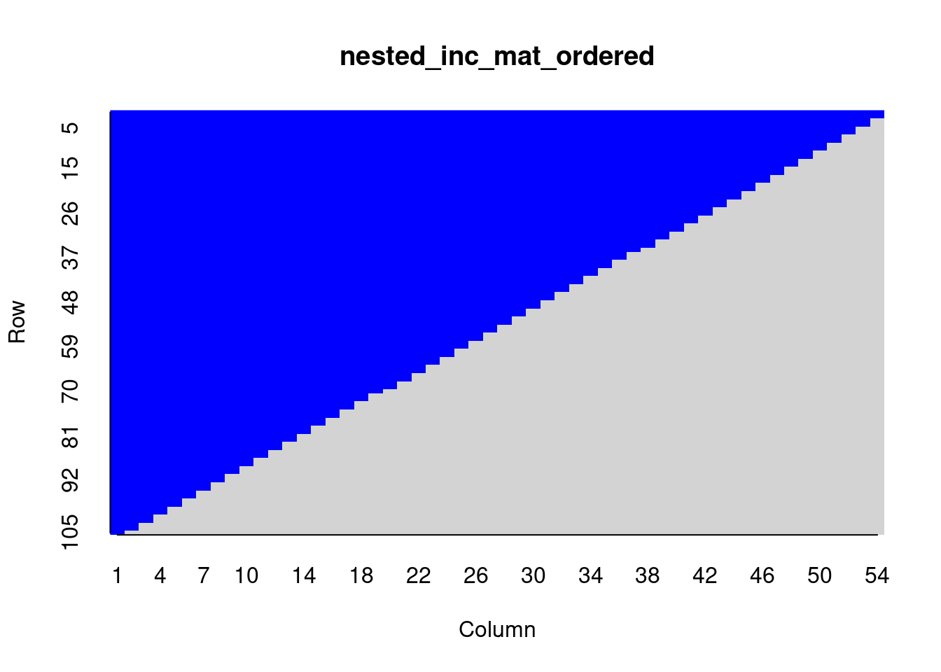
4.2.1 Exercise
Consider the following networks
- the empirical pollination network M_PL_026
- the perfectly nestsed network of the same dimensions as the network M_PL_026
- a randomized version of the network M_PL_026
The randomized network can be obtained using another function of the rweboflife package (you will hear more in the section on Null Models):
# load package
rnd_inc_mat <- rweboflife::null_model(M_PL_026_inc_mat, model = "equifrequent")
# order to be better visualized
rnd_inc_mat_ordered <- rnd_inc_mat[,order(colSums(rnd_inc_mat),decreasing = TRUE)]
# create a graph
rnd_graph <- graph_from_incidence_matrix(
  rnd_inc_mat,
  directed = FALSE,
  weighted = NULL,
  add.names = NULL
)
\(\bullet\) Visualize the three networks as a color-code matrix.
Hint: To prepare the empirical network for the vsualization, run the following code:
M_PL_026_inc_mat_ordered <- M_PL_026_inc_mat[,order(colSums(M_PL_026_inc_mat),decreasing = TRUE)]
colnames(M_PL_026_inc_mat_ordered) <- NULL
rownames(M_PL_026_inc_mat_ordered) <- NULL
\(\bullet\) Adapt the underlying code chunk to show the degree distributions \(P(k)\) of the three networks in the same plot:
M_PL_026_deg_dist <- degree_distribution_df(M_PL_026_graph)
nested_deg_dist <- degree_distribution_df( ??? )
rnd_deg_dist <- degree_distribution_df( ??? )

annotation_1 <- data.frame(
  x = 15,
  y = 0.9,
  label = "empirical M_PL_026 (circles)"
)
annotation_2 <- data.frame(
  x = 15,
  y = 0.7,
  label = "perfectly nested (squares)"
)
annotation_3 <- data.frame(
  x = 15,
  y = 0.5,
  label = "randomized (triangles)"
)

ggplot() +
  ggtitle("Degree distribution") +
  geom_point(data = M_PL_026_deg_dist, aes(k, frequency), shape = 21, size=2, color="black") +
  geom_point(data = nested_deg_dist, aes(k, frequency), shape = 22, size=2, color="dark green") +
  geom_point(data = rnd_deg_dist , aes(k, frequency), shape = 24, size=2, color="red") +
  # Add text
  geom_text(data=annotation_1, aes( x=x, y=y, label=label),
            color="black",
            size=4 , angle=0) +
  geom_text(data=annotation_2, aes( x=x, y=y, label=label),
            color="dark green",
            size=4 , angle=0) +
  geom_text(data=annotation_3, aes( x=x, y=y, label=label),
            color="red",
            size=4 , angle=0) +
  # # Add axes labels
  ylab(TeX("$P(k)$")) +
  xlab(TeX("$k$")) +
  coord_cartesian(xlim = c(0, 22), ylim = c(0.0001, 1.))
#scale_x_continuous(trans='log10') +
#scale_y_continuous(trans='log10')
\(\bullet\) Explain with your own workds why \(P(k)\) for the perfectly nested network is practically constant (think of the case of a square perfectly nested matrix). What major difference do you observe in relation to the other two degree distributions?
Hint: You may find it useful to comment the line coord_cartesian(...) and uncomment the following ones to display the graph in log-log scale.
\(\bullet\) Compute nestedness of the three networks using the function rweboflife::nestedness() and comment on the outcome.
4.3 Modularity
Let us download the network M_PA_002 from Web of life and create a bipartite igraph object from it (see session Toolkit for network analysis):
# Import the required packages
library(igraph)
library(dplyr)
library(rjson)
library(bipartite)
library(formattable)
# download the M_PA_002 network from the web-of-life API
json_url <- paste0("https://www.web-of-life.es/get_networks.php?network_name=M_PA_002")
M_PA_002_nw <- jsonlite::fromJSON(json_url)

# select the 3 relevant columns and create the igraph object
M_PA_002_graph <- M_PA_002_nw %>% select(species1, species2, connection_strength) %>%
  graph_from_data_frame(directed = FALSE)
# get info about species
my_info <- read.csv(paste0(base_url,"get_species_info.php?network_name=M_PA_002"))

isResource <- my_info$is.resource %>% as.logical() # 0/1 converted to FALSE/TRUE

# Add the "type" attribute to the vertices of the graph
V(M_PA_002_graph)$type <- !(isResource)
You can access object information using $:
## + 6/10 vertices, named, from 689ad0e:
## [1] Cecropia ficifolia    Cecropia membranacea  Cecropia engleriana
## [4] Cecropia polystachya Cecropia tessmannii Cecropia sp1 M_PA_002## + 13/13 edges from 689ad0e (vertex names):
## [1] Cecropia ficifolia --Azteca xanthochroa
## [2] Cecropia ficifolia --Camponotus balzani
## [3] Cecropia membranacea --Azteca ovaticeps
## [4] Cecropia membranacea --Azteca xanthochroa
## [5] Cecropia membranacea --Camponotus balzani
## [6] Cecropia engleriana --Azteca ovaticeps
## [7] Cecropia engleriana --Azteca xanthochroa
## [8] Cecropia polystachya --Azteca ovaticeps
## [9] Cecropia polystachya --Azteca xanthochroa
## [10] Cecropia polystachya --Camponotus balzani
## + ... omitted several edgesNow that we have the igraph object let’s compute its modularity. Sometimes the user may have a pre-defined node partitioning. If that is the case, we can manually define the modules if you already know which module which species belongs to.
# Manually define partitioning
membership = c(1,2,2,2,3,2,1,3,2,2)
# Compute modularity of partitioning
Q <- modularity(M_PA_002_graph, membership)
Q
## [1] 0.00887574We can also color the nodes according to the modules and plot the graph
# Color the nodes according to the modules
colbar <- rainbow(max(membership))
V(M_PA_002_graph)$color <- colbar[membership]

# Plot the graph
plot(M_PA_002_graph, layout=layout_with_fr, margin=0.0)
4.3.1 Community Detection
Some community detection algorithms available in igraph are:
- cluster_label_prop
- cluster_edge_betweenness
- cluster_fast_greedy
- cluster_leading_eigen
- cluster_optimal (SLOW!!)
Instead of having a predetermined idea of to which module each species belongs to, it is much more common to find the best partitioning of the nodes using one of the available community detection algorithms. Let us use the fast greedy algorithm:
## [1] 2 1 1 1 2 1 1 2 1 2Let’s get the modularity of the best partitioning.
## [1] 0.2218935Again, we can now color the nodes of our graph according the module they belong to.
colbar <- rainbow(max(modules$membership))
V(M_PA_002_graph)$color <- colbar[modules$membership]

plot(M_PA_002_graph,
     layout=layout_with_fr,
     vertex.size=12,
    #vertex.label=NA,
     margin=0.0)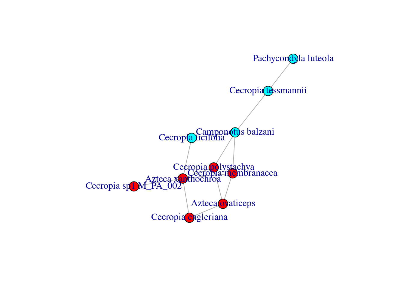
This layout makes much more sense!
4.3.2 Exercise
\(\bullet\) The node colors of the graph below represent a partitioning of the nodes into three modules.

Use the formula given in the lecture to compute the modularity Q associated with the partition (on paper).
Check your answer using R (on the R script in the workspace).
Do you think the given node partitioning is the best one, i.e. it optimizes Q? Provide arguments to support your answer.
Hint:
adj_matrix <- adj_matrix <- matrix(c(0, 0, 0, 0, 0, 0, 0,
                       0, 0, 0, 0, 0, 0, 0,
                       0, 0, 0, 0, 0, 0, 0,
                       0, 0, 0, 0, 0, 0, 0,
                       0, 0, 0, 0, 0, 0, 0,
                       0, 0, 0, 0, 0, 0, 0,
                       0, 0, 0, 0, 0, 0, 0),nrow=7,ncol=7)


graph <- graph_from_adjacency_matrix(adj_matrix,mode="undirected")

plot(graph,
     layout=layout_with_fr,
     vertex.size=12,
     vertex.label=NA,
     margin=0.0)
\(\bullet\) Download the network named M_SD_001 from Web of life using the usual sequence of commands, create an igraph object, and:
Use the community detection algorithm
cluster_louvain()to compute the optimal partitioning of nodes (modules) for that network.Compute the modularity M.
Plot the network coloring the nodes according to the modules they belong to and try to find the layout that better highlights communities.
Hint: To obtain a cleaner result, we recommend to remove the vertices names
You can then play with the size of nodes and with the layouts; a partial list of the last few is: layout_nicely, layout_with_kk, layout_randomly, layout_in_circle, layout_with_fr,layout_as_tree, layout_on_grid, layout_with_dh, layout_with_graphopt, layout_with_lgl, layout_with_mds, layout_with_sugiyama.