Chapter 1 Toolkit for network analysis
Fernando Pedraza
session 13/03/2025
An ecological network is a data set describing a group of species and their reciprocal interaction. Typically, this data is collected by ecologists in the field trough observations. Often, ecologists share their data sets to the wider scientific community. This valuable information then sparks additional research.
Some research groups have gathered network data sets from different publications and compiled them into public databases to facilitate access to the scientific community. Two of such examples are Mangal and Web of life.
In this session you will learn how to download datasets from the Web of life database of experimental ecological networks. You will also learn how to plot the networks and convert them into several formats that are suitable for further analysis.
1.1 Downloading data from the web of life
Web of life is a database of ecological networks developed and maintained by the Bascompte lab. You can find more information on the project in this paper or in this user’s manual.
When navigating to the Web of life you are greeted by a menu where you can select the type of species interactions you wish to access. After selecting a type of species interaction, you arrive at a world map which shows where the networks where collected. Each dot corresponds to a network and if you click on one, you will access the interaction data as well as some metadata —including the network name. Networks are named according to the following convention:
- Interaction type: mutualistic (M) or antagonistic (A)
- Network type: Plant-Ant (PAO), Plant-Epiphyte (PE), Pollination (PL), Seed Dispersal (SD), Food Webs (FW), Host-Parasite (HP), Host-Parasitoid (HPD), Plant-Herbivore (PH), Anemone-Fish (AF)
- Id labeling a specific network.
For example, the network M_PL_005 corresponds to a mutualistic network
of plant-pollinator interactions (with ID 5).
After clicking on a network, the web interface also allows you to
download the interaction data in various formats including .csv,
.xls, or .json. This is a useful tool if you want to inspect the
data. However, if you plan to analyse the data the database also allows
you to fetch data directly from R.
1.1.1 Download one network from the weboflife API
In a research projects it is often convenient to bypass the web
interface and store data directly in a data frame using the command
line. This has several advantages in terms of efficiency and
reproducibility of the analysis you are conducting. We will see how to
do this in R using the function fromJSON() of the package
jsonlite, but similar commands can be run in python or in other
languages.
In short, we will use the fromJSON() function to connect directly to
the Web of Life through a dedicated endpoint on the Application
Programming Interface (API).
Let us focus on network #1 of the Seed Dispersal type, in other words network M_SD_001. To download this network, we run the following commands:
# We begin by loading the jsonlite package
library(rjson)

# Now we download the network:

# First define the website we wish to connect to
base_url <- "https://www.web-of-life.es/"

# Next specify the network we wish to access
network_url <- "get_networks.php?network_name=M_SD_001"

# Then paste the base URL with the network URL
json_url <- paste0(base_url, network_url)

# Finally we use the fromJSON function from the jsonlite package to connect and fetch
# the data. I store the data in an object called M_SD_002_nw
M_SD_001_nw <- jsonlite::fromJSON(json_url)
Now that we have fetched the data we can investigate the type of object it is currently stored in on our system.
## [1] "data.frame"The data is stored as a data.frame thus we can use some commands to
quickly inspect the data set.
##   network_name              species1              species2 connection_strength
## 1     M_SD_001 Celastrus orbiculatus    Euphagus carolinus                   1
## 2     M_SD_001        Cornus florida Cardinalis cardinalis                   2
## 3     M_SD_001 Celastrus orbiculatus Cardinalis cardinalis                  13
## 4     M_SD_001       Lindera benzoin Cardinalis cardinalis                   1
## 5     M_SD_001   Smilax rotundifolia Cardinalis cardinalis                   6
## 6     M_SD_001     Lonicera japonica Cardinalis cardinalis                   2
It seems like we fetched the data correctly, however on close inspection
you will notice that the column connection_strength was downloaded as
character information. Since we will be using these numbers to build our
network, we need to convert the characters to numbers.
# Note that column "connection_strength" is read in as characters, however
# we need to convert them to numeric values. We can use the as.numeric()
# function to do this. We will also leverage the pipe operator (|>)
# and functions from the tidyverse package to make our code more
# concise and readable

# load the tidyverse package
library(tidyverse)

# convert the connection_strength column to numeric values
M_SD_001_nw <- M_SD_001_nw |>
  mutate(connection_strength = as.numeric(connection_strength))
Now that the data is stored in the correct format, we can leverage the
formattable package to display it (a bit nicer).
# load the formattable package
library(formattable)

# visualize the first few rows of the dataframe in nicer way
formattable(head(M_SD_001_nw))| network_name | species1 | species2 | connection_strength |
|---|---|---|---|
| M_SD_001 | Celastrus orbiculatus | Euphagus carolinus | 1 |
| M_SD_001 | Cornus florida | Cardinalis cardinalis | 2 |
| M_SD_001 | Celastrus orbiculatus | Cardinalis cardinalis | 13 |
| M_SD_001 | Lindera benzoin | Cardinalis cardinalis | 1 |
| M_SD_001 | Smilax rotundifolia | Cardinalis cardinalis | 6 |
| M_SD_001 | Lonicera japonica | Cardinalis cardinalis | 2 |
1.1.2 Download networks by type
You can download all networks of a particular type by accessing the
link: get_networks.php?interaction_type=NAMEOFINTERACTIONTYPE ,
where you can remove the placeholder text NAMEOFINTERACTIONTYPE and specify one of the available interaction types:
Anemone-Fish
FoodWebs
Host-Parasite
Plant-Ant
Plant-Herbivore
Pollination
SeedDispersal
To download all Seed Dispersal networks, we would run the following commands:
# Specify the network type we wish to access
network_url <- "get_networks.php?interaction_type=SeedDispersal"

# Paste the base URL with the network URL
json_url <- paste0(base_url, network_url)

# Use the fromJSON function from the jsonlite package to connect and fetch
# the data. I store the data in an object called sd_nws
sd_nws <- jsonlite::fromJSON(json_url)
As before, we need to change the data in the connection_strength from
character to numeric.
# convert data in connection_strength column from character to numeric
sd_nws <- sd_nws |>
  mutate(connection_strength = as.numeric(connection_strength))
Let’s take a look at the data we downloaded:
| network_name | species1 | species2 | connection_strength |
|---|---|---|---|
| M_SD_031 | Laurus azorica | Turdus merula | 4 |
| M_SD_031 | Sonchus tenerrimus | Carduelis carduelis | 1 |
| M_SD_031 | Fragaria vesca | Turdus merula | 3 |
| M_SD_031 | Fragaria vesca | Sylvia atricapilla | 4 |
| M_SD_031 | Calluna vulgaris | Turdus merula | 1 |
| M_SD_031 | Calluna vulgaris | Sylvia atricapilla | 1 |
We can leverage some base R commands to list the names of all the seed dispersal network we downloaded.
##  [1] "M_SD_031" "M_SD_025" "M_SD_011" "M_SD_001" "M_SD_002" "M_SD_003"
##  [7] "M_SD_004" "M_SD_005" "M_SD_006" "M_SD_007" "M_SD_008" "M_SD_009"
## [13] "M_SD_010" "M_SD_012" "M_SD_013" "M_SD_014" "M_SD_015" "M_SD_016"
## [19] "M_SD_017" "M_SD_018" "M_SD_019" "M_SD_020" "M_SD_021" "M_SD_022"
## [25] "M_SD_023" "M_SD_024" "M_SD_026" "M_SD_027" "M_SD_028" "M_SD_029"
## [31] "M_SD_030" "M_SD_032" "M_SD_033" "M_SD_034"
We can also then extract the information for a particular network of
interest, for example M_SD_028. For this, we can leverage commands
from the tidyverse package.
# from the dataframe containing all SD networks
sd_nws |>
  # keep only observations from the network "M_SD_028"
  dplyr::filter(network_name == "M_SD_028") |>
  # display the information in a nice way
formattable()| network_name | species1 | species2 | connection_strength |
|---|---|---|---|
| M_SD_028 | Crataegus monogyna | Turdus merula | 1 |
| M_SD_028 | Hedera helix | Turdus merula | 1 |
| M_SD_028 | Berberis vulgaris | Turdus merula | 1 |
| M_SD_028 | Lonicera arborea | Turdus merula | 1 |
| M_SD_028 | Rosa canina | Turdus merula | 1 |
| M_SD_028 | Taxus baccata | Turdus merula | 1 |
| M_SD_028 | Crataegus monogyna | Turdus philomelos | 1 |
| M_SD_028 | Berberis vulgaris | Turdus philomelos | 1 |
| M_SD_028 | Crataegus monogyna | Turdus iliacus | 1 |
| M_SD_028 | Hedera helix | Turdus iliacus | 1 |
| M_SD_028 | Berberis vulgaris | Turdus iliacus | 1 |
| M_SD_028 | Taxus baccata | Turdus iliacus | 1 |
| M_SD_028 | Crataegus monogyna | Turdus torquatus | 1 |
| M_SD_028 | Hedera helix | Turdus torquatus | 1 |
| M_SD_028 | Berberis vulgaris | Turdus torquatus | 1 |
| M_SD_028 | Juniperus communis | Turdus torquatus | 1 |
| M_SD_028 | Lonicera arborea | Turdus torquatus | 1 |
| M_SD_028 | Rosa canina | Turdus torquatus | 1 |
| M_SD_028 | Taxus baccata | Turdus torquatus | 1 |
| M_SD_028 | Viscum album | Turdus torquatus | 1 |
| M_SD_028 | Crataegus monogyna | Turdus viscivorus | 1 |
| M_SD_028 | Hedera helix | Turdus viscivorus | 1 |
| M_SD_028 | Berberis vulgaris | Turdus viscivorus | 1 |
| M_SD_028 | Rosa canina | Turdus viscivorus | 1 |
| M_SD_028 | Taxus baccata | Turdus viscivorus | 1 |
| M_SD_028 | Viscum album | Turdus viscivorus | 1 |
1.1.3 Download all networks
You can also download all networks from the Web of Life by not
specifying an interaction_type:
# Specify the network type we wish to access
network_url <- "get_networks.php"

# Paste the base URL with the network URL
json_url <- paste0(base_url, network_url)

# Use the fromJSON function from the jsonlite package to connect and fetch
# the data. I store the data in an object called all_nws
all_nws <- jsonlite::fromJSON(json_url)
Remember to change the data in the connection_strength from character
to numeric!
# convert data in connection_strength column from character to numeric
all_nws <- all_nws |>
  mutate(connection_strength = as.numeric(connection_strength))
With the entire data set in hand, we can once again use the tidyverse
package to filter out relevant information. Here are two such examples.
Obtain all networks corresponding to antagonistic interactions:
# from the object containing all networks
all_antagonistic_nws <- all_nws |>
  # keep only those for which the network name contains "A_"
  dplyr::filter(str_detect(network_name, 'A_'))

# check the names of the resulting dataframe
unique(all_antagonistic_nws$network_name)
## [1] "A_HP_001" "A_HP_002" "A_HP_003" "A_HP_004" "A_HP_005" "A_HP_006" ## [7] "A_HP_007" "A_HP_008" "A_HP_009" "A_HP_010" "A_HP_011" "A_HP_012" ## [13] "A_HP_013" "A_HP_014" "A_HP_015" "A_HP_016" "A_HP_017" "A_HP_018" ## [19] "A_HP_019" "A_HP_020" "A_HP_021" "A_HP_022" "A_HP_023" "A_HP_024" ## [25] "A_HP_025" "A_HP_026" "A_HP_027" "A_HP_028" "A_HP_029" "A_HP_030" ## [31] "A_HP_031" "A_HP_032" "A_HP_033" "A_HP_034" "A_HP_035" "A_HP_036" ## [37] "A_HP_037" "A_HP_038" "A_HP_039" "A_HP_040" "A_HP_041" "A_HP_042" ## [43] "A_HP_043" "A_HP_044" "A_HP_045" "A_HP_046" "A_HP_047" "A_HP_048" ## [49] "A_HP_049" "A_HP_050" "A_HP_051" "A_PH_001" "A_PH_002" "A_PH_003" ## [55] "M_PA_002" "M_PA_005" "A_PH_004" "A_PH_005" "A_PH_006" "A_PH_007" ## [61] "M_PA_003" "M_PA_001" "M_PA_004"Obtain all food webs:
    # from the object containing all networks
    all_foodweb_nws <- all_nws |>
      # keep only those that corrspond to food webs
      dplyr::filter(str_detect(network_name, 'FW_'))

    # check the names of the resulting dataframe
    unique(all_foodweb_nws$network_name)
## [1] "FW_002" "FW_003" "FW_004" "FW_005" "FW_006" "FW_007"
## [7] "FW_009" "FW_010" "FW_011" "FW_012_01" "FW_012_02" "FW_013_01"
## [13] "FW_013_02" "FW_013_03" "FW_013_04" "FW_013_05" "FW_014_01" "FW_014_02"
## [19] "FW_014_03" "FW_014_04" "FW_015_01" "FW_015_02" "FW_015_03" "FW_015_04"
## [25] "FW_016_01" "FW_017_01" "FW_017_02" "FW_017_03" "FW_017_04" "FW_017_05"
## [31] "FW_017_06" "FW_001" "FW_008"1.2 Build and visualise networks
After downloading the data from the web of life, we will now convert it
into a network. To do so in R, we will use the igraph package. This
package contains many useful functions to build, analyse, and visualise
networks. However, it is important to note that this package was
developed to study networks as mathematical objects. As a result, there
are some slight differences in the terminology that the package uses and
the concepts you will cover during this course. Here, I provide a
(very!) brief overview of the most important differences.
Graph Theory is a branch of mathematics that studies graphs —mathematical structures used to describe pairwise relations between objects. In turn, Network Science is an academic study that describes the connections between distinct elements (e.g. computer networks, social networks, ecological networks, etc.). Thus, the object of study for Graph Theory and Network Science is the same. Yet, they use different terminology:
| Graph Theory | Network Science |
|---|---|
| graph | network |
| vertex | node |
| edge | link |
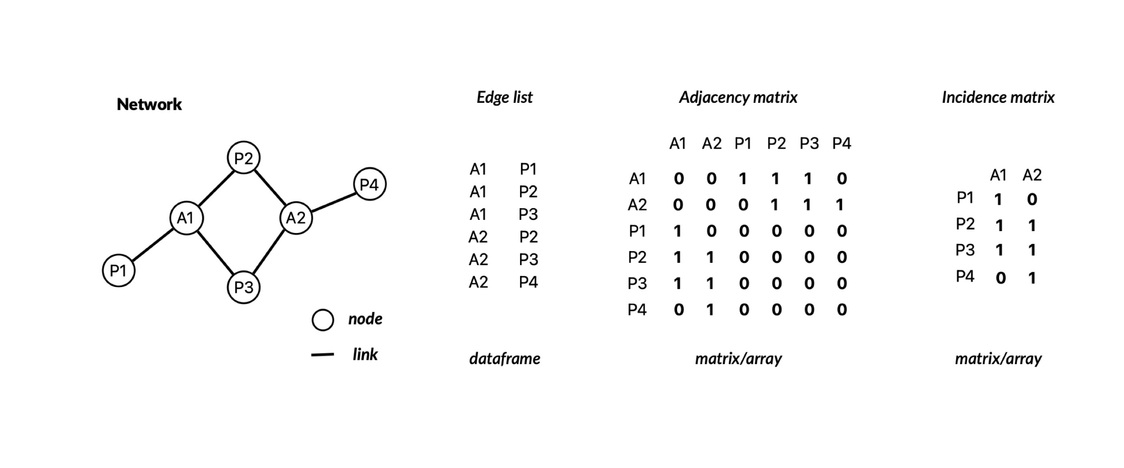
The data describing the interaction between elements can be represented in several ways. For example, as a network, edge list, adjacency matrix or incidence matrix.
These representations can be stored in R as different data structures
such as matrices or arrays. In addition, the igraph package has a
special type of object which allows you to store networks.
| Representation | Data structure |
|---|---|
| edge list | dataframe |
| network | igraph (igraph object) |
| adjacency matrix | matrix/array |
| incidence matrix | matrix/array |
1.2.1 From edge list to network
The network data we download from
Web of Life is
stored as a data.frame. It consists of four columns: network_name,
species1, species2, and connection_strength. Thus, the
interactions are stored as an edge list and we can leverage the last
three columns to construct the network.
Let’s illustrate this for the network M_PL_036. We will: 1) download
the data from the web of life, 2) discard the network_name column, 3)
convert the connection_strength column to numeric, and 4) get a
glimpse of the data.
# 1 Download network M_PL_036.

# First define the website we wish to connect to
base_url <- "https://www.web-of-life.es/"

# Next specify the network we wish to access
network_url <- "get_networks.php?network_name=M_PL_036"

# Then paste the base URL with the network URL
json_url <- paste0(base_url, network_url)

# Finally we use the fromJSON function from the jsonlite
# package to connect and fetch the data.
# I store the data in an object called M_PL_036_nw
M_PL_036_nw <- jsonlite::fromJSON(json_url)

# 2 Discard the network_name column
M_PL_036_nw <- M_PL_036_nw |>
  select(species1, species2, connection_strength)

# 3 Convert the connection_strength column to numeric
M_PL_036_nw <- M_PL_036_nw |>
  mutate(connection_strength = as.numeric(connection_strength))

# 4 Get a glimpse of the data
head(M_PL_036_nw)
## species1 species2 connection_strength
## 1 Lotus corniculatus Apis mellifera 1
## 2 Azorina vidalii Apis mellifera 1
## 3 Reseada luteola Apis mellifera 1
## 4 Leucanthemum vulgare Hymenoptera sp1 M_PL_036 1
## 5 Daucus carota Hymenoptera sp1 M_PL_036 1
## 6 Azorina vidalii Hymenoptera sp1 M_PL_036 1Now we can use the function graph_from_data_frame() from the igraph
package to turn our data.frame (edge list) into a network object.
# Load the igraph package
library(igraph)

# Create the network using our data
M_PL_036_network <- graph_from_data_frame(M_PL_036_nw, directed = FALSE)

# Take a glimpse at the object
M_PL_036_network
## IGRAPH e825b62 UN-- 22 30 --
## + attr: name (v/c), connection_strength (e/n)
## + edges from e825b62 (vertex names):
## [1] Lotus corniculatus --Apis mellifera
## [2] Azorina vidalii --Apis mellifera
## [3] Reseada luteola --Apis mellifera
## [4] Leucanthemum vulgare --Hymenoptera sp1 M_PL_036
## [5] Daucus carota --Hymenoptera sp1 M_PL_036
## [6] Azorina vidalii --Hymenoptera sp1 M_PL_036
## [7] Silene vulgaris --Hymenoptera sp1 M_PL_036
## [8] Solidago sempervirens--Hymenoptera sp1 M_PL_036
## + ... omitted several edgesAs you can see from the last command, we have just created an igraph
object. Note that for this plant-pollinator network, it is not necessary
to know who pollinates whom. This is why we passed the additional
argument directed = FALSE to the graph_from_data_frame() function.
However, who is whom is important to denote when building a food web.
For such cases, we would pass directed = TRUE.
1.2.2 Plotting the network
Once the network is represented as an igraph object it can easily be
visualized using the plot function. I demonstrate this next and also
include some extra arguments to tweak the look of the network (for a
more thorough description of the arguments that the plot function can
handle please consult this
webpage).
plot(M_PL_036_network, # the name of the igraph object
     vertex.size=4, # the size of the nodes/vertices
     vertex.label=NA, # if the nodes/vertices should be named
     edge.size= 0.3, # the size of the links/edges
     layout = layout_randomly)  # how the nodes should be arranged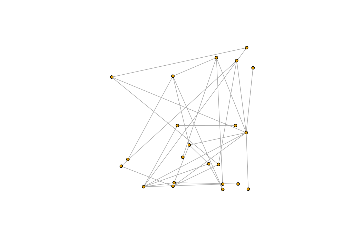
Other possible layouts of the links and nodes are: layout_nicely,
layout_with_kk, layout_randomly, layout_in_circle,
layout_on_sphere, etc. (you can find a complete list
here).
1.2.3 Creating a bipartite network
Bipartite networks are a particular type of network where nodes can be classified into two groups and connections only occur between elements belonging to different groups Pollination networks are one such example, where species are either plants or animals and interactions only occur between them.
Igraph does not by default determine whether a network is bipartite.
Instead, we have to run a specific function (bipartite.mapping()) to
determine whether the network could be bipartite —whether the nodes can
be classified into two groups such that nodes of the same group do not
interact. Next, I will demonstrate how to construct a bipartite network
out of the interaction data from M_PL_036_nw (the pollination network
we downloaded before).
# (Again) I create the network using our data
M_PL_036_network <- graph_from_data_frame(M_PL_036_nw, directed = FALSE)

# Determine whether the network could be bipartite
bipartite_res <- bipartite.mapping(M_PL_036_network)

# Take a look at the output
# $res: Determines whether the network could be bipartite (TRUE/FALSE)
# $type If res is TRUE, then each node is classified into a group.
bipartite_res
## $res
## [1] TRUE
##
## $type
## [1] FALSE FALSE FALSE FALSE FALSE FALSE FALSE FALSE FALSE FALSE TRUE TRUE
## [13] TRUE TRUE TRUE TRUE TRUE TRUE TRUE TRUE TRUE TRUEFrom this, we can conclude that our network can indeed be bipartite
($res is TRUE) and we now the group that each node belongs to (the
vector from $type). To make our network bipartite, we have to add an
attribute to each node that specifies the type of node it is (i.e. the
group that it belongs to). Thus, we can use the group classification
from bipartite_res$type to assign the node type attribute:
# Add a "type" attribute to the nodes (vertices) of the network.
# Each node's type is assigned using the bipartite.mapping obtained
# in the previous code block.
V(M_PL_036_network)$type <- bipartite_res$type
By assigning the nodes (i.e. vertices) a type attribute, we have
transformed the network to be bipartite. We can confirm this by running
the command is_bipartite .
## [1] TRUENow our network is bipartite and each node has been assigned to one of two groups. But which group corresponds to plants or animals? For now, we can check this by accessing the name of the first species stored in the network and then access the group it belongs to.
## + 1/22 vertex, named, from 333977b:
## [1] Lotus corniculatus
Lotus corniculatus is a plant. Let’s check which group it was assigned to.
## [1] FALSELotus corniculatus belongs to group FALSE. Thus, the node type is
telling us whether the node is an animal. In other words, all nodes that
are plants are FALSE and all nodes that are animals are TRUE.
1.2.4 From a bipartite network to adjacency matrix
We can represent a network (either uniparite or bipartite) as an adjacency matrix —a square matrix whose elements indicate whether two nodes interact with one another (in other words, if two elements are adjacent). The elements of the adjacency matrix of an unweighted network can take values of 0 (if no interaction occurs) or 1 (if an interaction occurs). In the case of weighted networks, the matrix contains the frequency of the interactions (e.g. the number of visitation events by a pollinator).
To obtain the adjacency matrix of a network we can use the
as_adjacency_matrix() function from the igraph package.
# convert our bipartite network into an adjacency matrix
M_PL_036_adjacency <- as_adjacency_matrix(M_PL_036_network, sparse = FALSE)
# we set sparse to false so that elements without interactions
# are coded as 0
Let’s take a look at the size of the resulting matrix:
## [1] 22 22We have a 22x22 adjacency matrix, meaning that our network contains 22 species in total (animals and plants combined). This is inline with our data in its network representation:
## + 22/22 vertices, named, from 333977b:
##  [1] Lotus corniculatus        Azorina vidalii
##  [3] Reseada luteola           Leucanthemum vulgare
##  [5] Daucus carota             Silene vulgaris
##  [7] Solidago sempervirens     Crithmum maritimum
##  [9] Beta maritima             Freesia sp1 M_PL_036
## [11] Apis mellifera            Hymenoptera sp1 M_PL_036
## [13] Unidentified sp2 M_PL_036 Unidentified sp3 M_PL_036
## [15] Bombus sp1 M_PL_036       Lepidoptera sp4 M_PL_036
## [17] Lucilia sp1 M_PL_036      Unidentified sp5 M_PL_036
## [19] Calliphora sp1 M_PL_036   Unidentified sp6 M_PL_036
## + ... omitted several vertices
It’s important to know how to build an adjacency matrix from a network
since some network analysis (which you will learn about during the
course) require you to work with the adjacency matrix representation of
the network. Moreover, you can also visualise a network in its adjacency
matrix representation using the bipartite package:
# Load the bipartite package
library(bipartite)
# Visualise the adjacency matrix
plotmatrix(M_PL_036_adjacency, plot_labels = TRUE) # note that to fine tune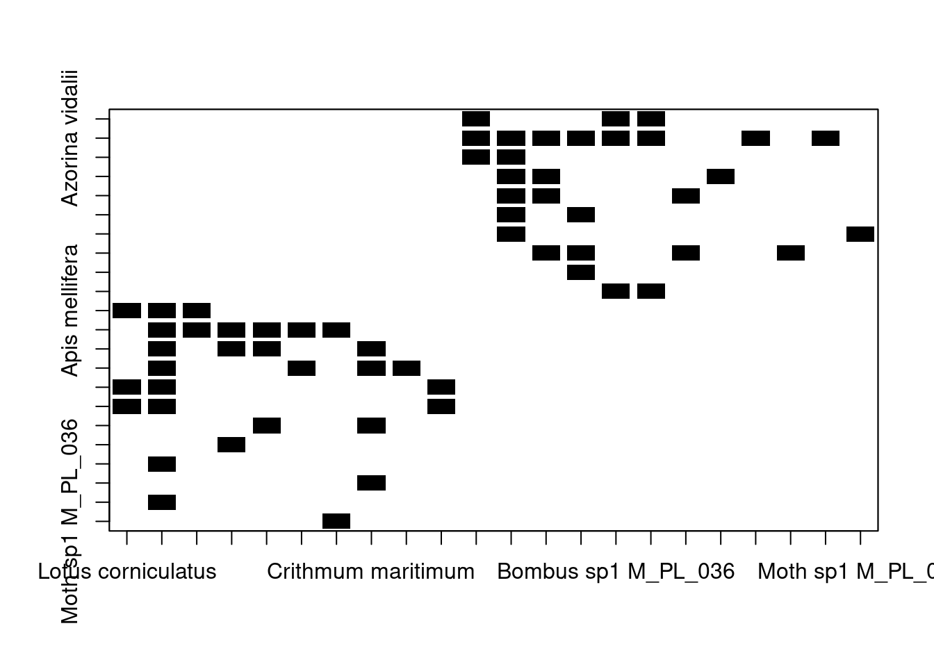
1.2.5 From a bipartite network to incidence matrix
We can represent a network as an incidence matrix —a matrix whose elements indicate the relationship between two classes of elements (such as the groups of bipartite networks). The elements of the incidence matrix of an unweighted network can take values of 0 (if no interaction occurs) or 1 (if an interaction occurs). In the case of weighted networks, the matrix contains the frequency of the interactions (e.g. the number of visitation events by a pollinator).
To obtain the incidence matrix of a network we can use the
as_incidence_matrix() function from the igraph package.
# convert our bipartite network into an incidence matrix
M_PL_036_incidence <- as_incidence_matrix(M_PL_036_network, sparse = FALSE)
# we set sparse to false so that elements without interactions
# are coded as 0
Let’s take a look at the size of the resulting matrix:
## [1] 10 12We have a 10x12 adjacency matrix, meaning that our network contains 10 species belonging to one group and 12 to the other group. This is inline with our data in its network representation:
##  [1] FALSE FALSE FALSE FALSE FALSE FALSE FALSE FALSE FALSE FALSE  TRUE  TRUE
## [13]  TRUE  TRUE  TRUE  TRUE  TRUE  TRUE  TRUE  TRUE  TRUE  TRUE
We have 10 plants (type == FALSE) and 12 animals (type == TRUE).
It’s important to know how to build an incidence matrix from a network
since some network analysis (which you will learn about during the
course) require you to work with the incidence matrix representation of
the network. Moreover, you can also visualise a network in its incidence
matrix representation using the bipartite package:
# Visualise the incidence matrix
plotmatrix(M_PL_036_incidence, plot_labels = TRUE) # note that to fine tune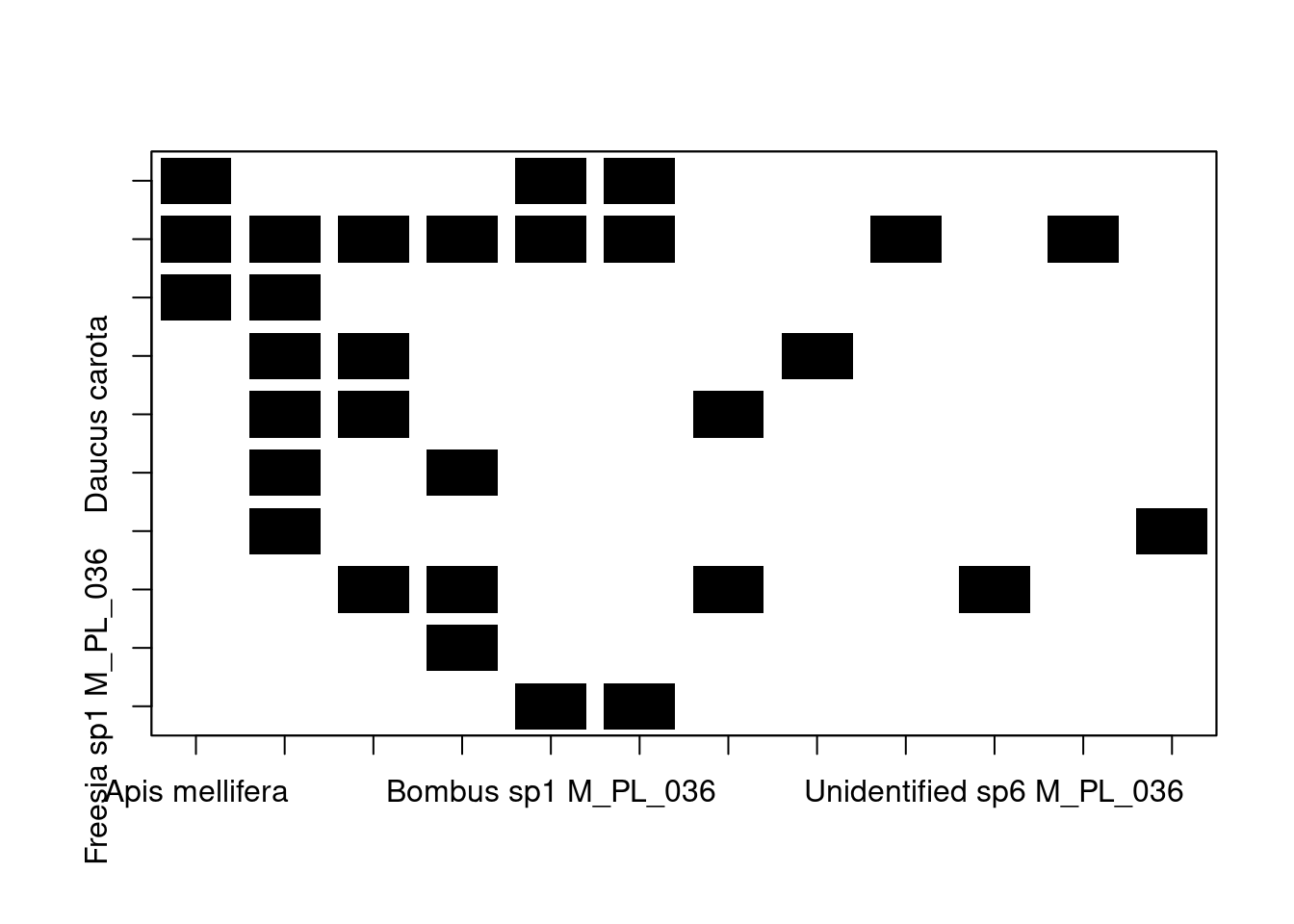
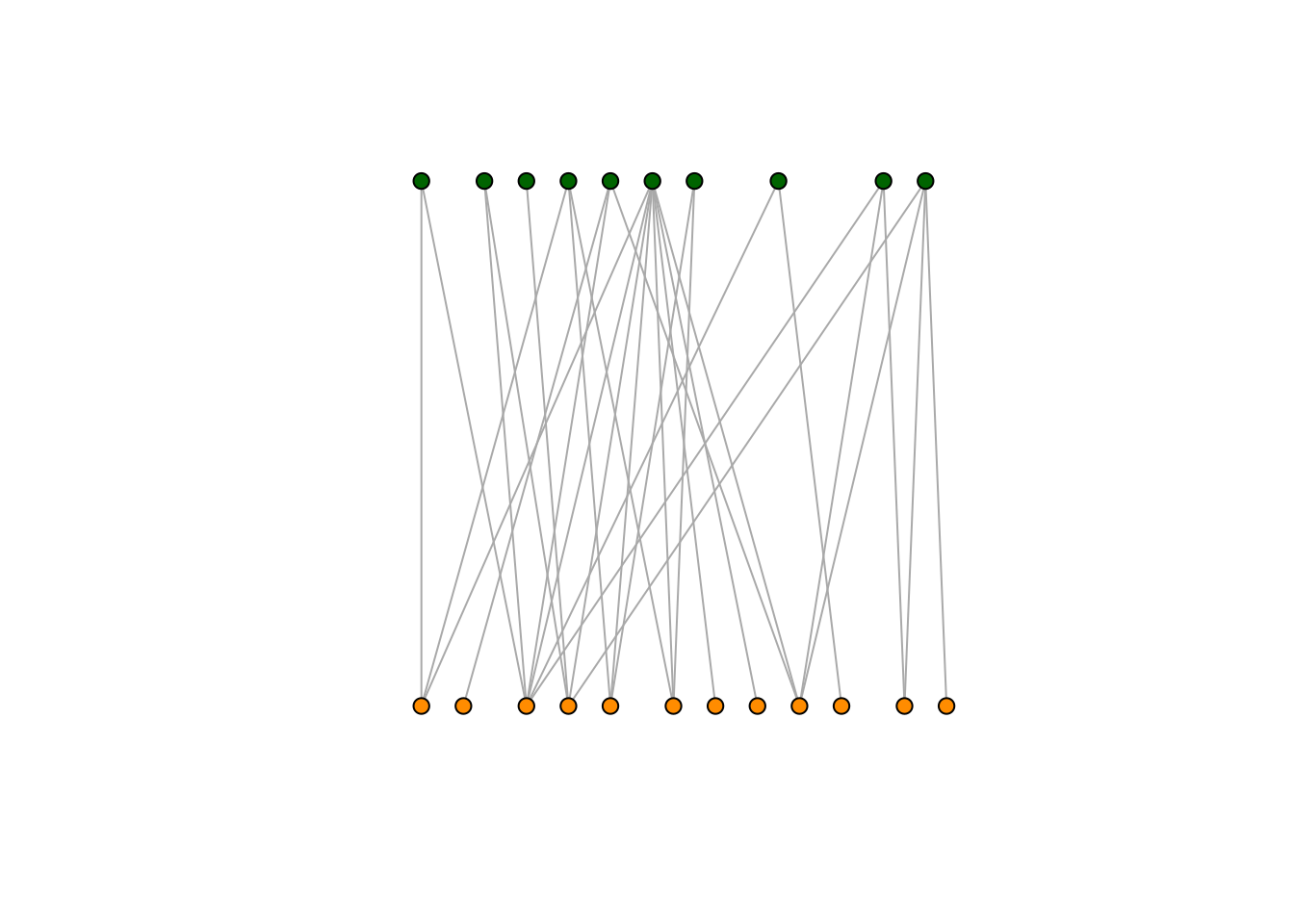
1.2.6 Plotting a bipartite network
Finally, we can also plot our bipartite network as before using the
plot function. However, this time we colour the nodes depending on the
group they belong to. Here all plant nodes will be coloured green and
all animal nodes will be orange. Moreover, we use a layout specifically
designed for bipartite networks:
plot(M_PL_036_network,
     layout = layout_as_bipartite,# layout designed for bipartite networks
     vertex.color=c("darkgreen","darkorange")[V(M_PL_036_network)$type+1],
     # color nodes depending on the group that they belong to
     vertex.size = 6, # the size of the nodes/vertices
     vertex.label = NA, # if the nodes/vertices should be named
     edge.size = 0.3
     )
The bipartite package also has functions for visualising bipartite networks. However, what we pass to the plotting functions is the incidence matrix (not the igraph object as before!).
plotweb(M_PL_036_incidence,
        text.rot=90,
        bor.col.interaction="gray40",plot.axes=F,
        col.high="darkorange",
        col.low="darkgreen",
        y.lim=c(-1,3))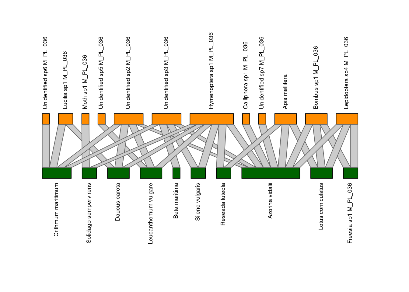
1.3 Exercise
In this section you will put in practice the workflow demonstrated in the previous sections. Your tasks are:
Download all the Pollination network data from the Web of Life using the commands shown above.
From the downloaded data, select one pollination network and convert the data from an edge list into a bipartite network using the
igraphpackage.Plot the bipartite network using the
bipartitepackage.Convert the bipartite network into an incidence matrix and plot the matrix using the
bipartitepackage.
1.4 Solutions
- Download all the Pollination network data from the Web of Life using the commands shown above.
# Specify the network type we wish to access
network_url <- "get_networks.php?interaction_type=Pollination"

# Define the website we wish to connect to
base_url <- "https://www.web-of-life.es/"

# Paste the base URL with the network URL
json_url <- paste0(base_url, network_url)

# Use the fromJSON function from the jsonlite package to connect and fetch
# the data. I store the data in an object called pollination_nws
pollination_nws <- jsonlite::fromJSON(json_url)

# I print out the first few rows of the data
head(pollination_nws)
## network_name species1 species2 connection_strength
## 1 M_PL_063 Lantana camara Phaethornis eurynome 1
## 2 M_PL_063 Lantana camara Stephanoxis lalandi 26
## 3 M_PL_063 Fuchsia regia Phaethornis eurynome 6
## 4 M_PL_063 Fuchsia regia Thalurania glaucopis 5
## 5 M_PL_063 Fuchsia regia Clytolaema rubricauda 15
## 6 M_PL_063 Psychotria leiocarpa Thalurania glaucopis 2- From the downloaded data, select one pollination network and convert the data
from an edge list into a bipartite network using the
igraphpackage.
# I will select network M_PL_042 from the data frame containing all pollination
# networks and convert the connection_strength column to numeric data
my_edge_data <- pollination_nws |>
  # Keep only observations from the network "M_PL_042"
  dplyr::filter(network_name == "M_PL_042") |>
  # Keep only relevant columns
  dplyr::select(species1, species2, connection_strength) |>
  # Convert the connection_strength column data to numeric
  mutate(connection_strength = as.numeric(connection_strength))

# Convert the edge data into a network using igraph
my_network <- graph_from_data_frame(my_edge_data, directed = FALSE)

# Determine if network can be bipartite
my_bipartite_res <- bipartite.mapping(my_network)

# Extract groups and assign them to the nodes in the network to make it bipartite
V(my_network)$type <- my_bipartite_res$type

# Check if network is bipartite
is_bipartite(my_network)
## [1] TRUE- Plot the bipartite network using the
bipartitepackage.
# First convert network to incidence matrix
my_incidence <- as_incidence_matrix(my_network, sparse = FALSE)

# Plot the network
plotweb(my_incidence,
        text.rot=90,
        bor.col.interaction="gray40",plot.axes=F,
        col.high="darkorange",
        col.low="darkgreen",
        y.lim=c(-1,3))
- Convert the bipartite network into an incidence matrix and plot the
matrix using the
bipartitepackage.
# We already converted the network to an incidence matrix (see previous exercise),
# so we can directly visualise the matrix
plotmatrix(my_incidence, plot_labels = FALSE)