Chapter 2 Measuring modularity
Fernando Pedraza
session 14/03/2025
In this session, we will cover how to measure the modularity of an ecological network. First, you will build networks and quantify modularity “by hand” and then you will learn the necessary commands to replicate the analysis in R. We will continue working with networks from the Web of Life, so we will reuse some concepts and commands from the previous session (Toolkit for network analysis).
2.1 Networks and modularity by hand
As a warm up, we begin by reviewing some concepts that have already been introduced in past lectures and exercise sessions. Namely, species degree and adjacency matrix. As a quick refresh:
In the case of ecological networks, the degree of a species refers to how many species it interacts with.
The adjacency matrix is a square matrix whose elements indicate whether two nodes interact with one another (in other words, if two elements are adjacent).
Exercise 1
For the graph drawn below:
- Write down the degree of each node.
- Compute its adjacency matrix.
Please solve this exercise on a piece of paper. When you have finished, take a picture of your solution and upload it (along with the rest of your submission) into the corresponding folder on OLAT.
Exercise 2
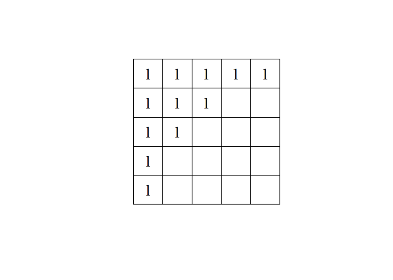
Draw the graph represented by the following adjacency matrix:
\[ \\A = \begin{bmatrix} 0 & 0 & 1 & 0 & 1 \\ 0 & 0 & 0 & 1 & 1 \\ 1 & 0 & 0 & 0 & 0 \\ 0 & 1 & 0 & 0 & 1 \\ 1 & 1 & 0 & 1 & 0 \\ \end{bmatrix} \] Please solve this exercise on a piece of paper. When you have finished, take a picture of your solution and upload it (along with the rest of your submission) into the corresponding folder on OLAT.
Exercise 3
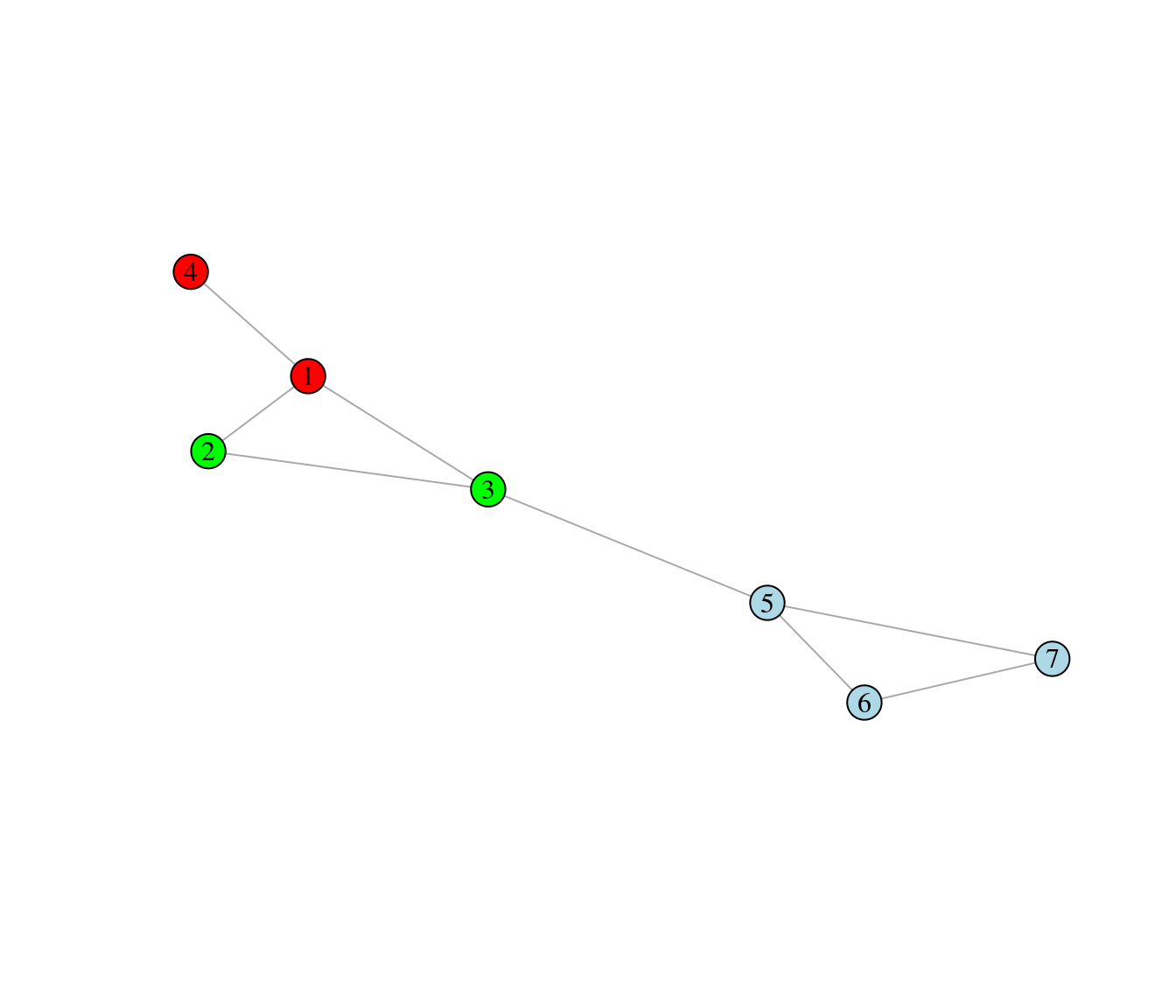
The node colors of the graph below represent a partitioning of the nodes into three modules.
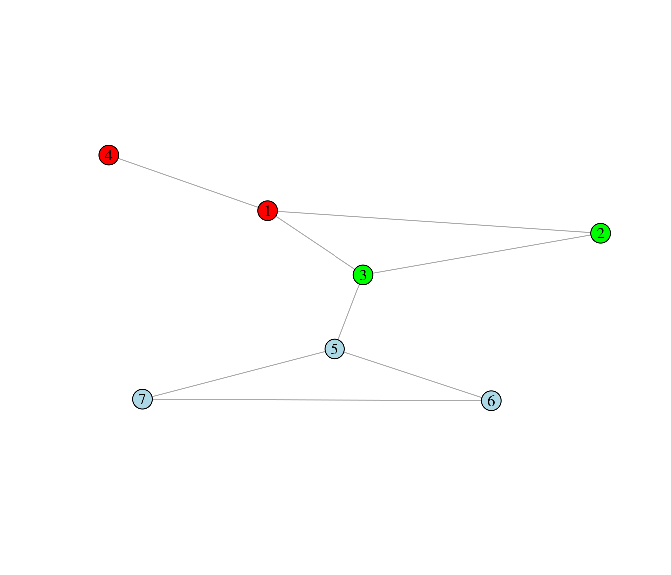
Use the formula given in the Food Webs lecture to compute the modularity associated with the partition.
\[ M = \sum_{\text{all modules s}}\left[\frac{l_s}{L} - \left(\frac{d_s}{2L}\right)^2\right], \]
where \(l_s\) is the number of interactions inside module \(s\), \(L\) is the number of interactions in the whole network, and \(d_s\) is the sum of the species’ degree inside module \(s\).
Do you think the given node partitioning is the best, i.e. it optimizes modularity (argue)?
2.2 Computing modularity in R
We will now use R to quantify modularity. Let’s start by loading some packages:
# Import the required libraries
library(rjson) # used for downloading networks from the Web of Life
library(igraph) # used for finding node partitions and plotting networks
library(tidyverse) # used for wrangling data sets
library(bipartite) # used for plotting networks
Next we will download a pollination network (M_PL_008) from the Web of
Life, using the workflow outlined in the Toolkit for network analysis
chapter.
# Download the M_PL_008 network from the web-of-life
json_url <- paste0("https://www.web-of-life.es/get_networks.php?network_name=M_PL_008")
M_PL_008_nw <- jsonlite::fromJSON(json_url)

# Keep only the three relevant columns and use them to create the network
M_PL_008_graph <- M_PL_008_nw |>
  dplyr::select(species1, species2, connection_strength) |>
  # convert the connection_strength column to numeric
  mutate(connection_strength = as.numeric(connection_strength)) |>
  graph_from_data_frame(directed = FALSE)

# Get a glimpse at the network
M_PL_008_graph
## IGRAPH 5ba9a00 UN-- 49 106 --
## + attr: name (v/c), connection_strength (e/n)
## + edges from 5ba9a00 (vertex names):
## [1] Echium wildpretii --Eristalis tenax
## [2] Pimpinella cumbrae --Eristalis tenax
## [3] Pterocephalus lasiospermus--Eristalis tenax
## [4] Mentha longifolia --Eristalis tenax
## [5] Tolpis webbii --Eristalis tenax
## [6] Echium wildpretii --Apis mellifera
## [7] Pimpinella cumbrae --Apis mellifera
## [8] Pterocephalus lasiospermus--Apis mellifera
## + ... omitted several edgesWe have now created the network, but since this is a pollination network we need to convert it into a bipartite network. At the moment it is a unipartite network:
## [1] FALSEIn the last session, we used igraph to determine the group that each species belongs to (i.e. plant or pollinator). Luckily, the web of life already contains this information. We can download this information for any network, along with other taxonomic data using the following command:
# Download taxonomic data from the Web of Life for our downloaded network
# In this case we specify network_name=M_PL_008
taxonomic_data_M_PL_008 <- read.csv(
  paste0("https://www.web-of-life.es/","get_species_info.php?network_name=M_PL_008"))

head(taxonomic_data_M_PL_008)
## species abundance role is.resource taxonomic.resolution
## 1 Eristalis tenax NA Pollinator 0 Species
## 2 Apis mellifera NA Pollinator 0 Species
## 3 Anthophora alluaudi NA Pollinator 0 Genus
## 4 Megachile canariensis NA Pollinator 0
## 5 Euodynerus reflexus NA Pollinator 0
## 6 Anastoechus latifrons NA Pollinator 0 Family
## kingdom order family
## 1 Animals Diptera Syrphidae
## 2 Animals Hymenoptera Apidae
## 3 Animals Hymenoptera Apidae
## 4 Animals Hymenoptera Megachilidae
## 5 Animals Hymenoptera Eumenidae
## 6 Animals Diptera BombyliidaeThe column is.resource denotes whether a species is a resource (i.e. a
plant) or not. So, we can use this column to assign each species in the
network to a group and thus make the network bipartite. However (!) the
order of the species names is different to the order of the names of the
species in the network. So we must make sure that we are extracting the
accurate information!
# First reorder the taxonomic data so that it follows
# the same order of species as the network we created
taxonomic_data_M_PL_008 <- taxonomic_data_M_PL_008[match(names(V(M_PL_008_graph)),
taxonomic_data_M_PL_008$species), ]

# Extract the information from the is.resource column
isResource <- as.logical(taxonomic_data_M_PL_008$is.resource) # change to T/F
# Add the "type" attribute to the nodes of the graph
V(M_PL_008_graph)$type <- !(isResource)
Now that we have assigned a type to each node, the network is of type bipartite.
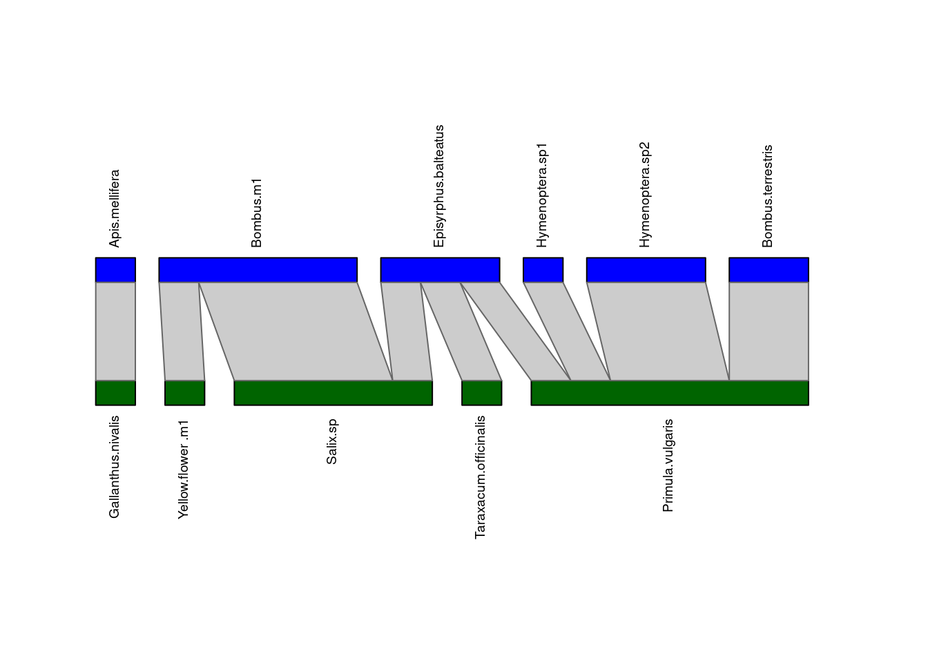
## [1] TRUESince this is a bipartite network, let’s create the incidence matrix and
use the bipartite package to plot it.
# Convert the igraph object into an incidence matrix
M_PL_008_incidence <- as_incidence_matrix(M_PL_008_graph, sparse = FALSE)

# Plot using bipartite
plotweb(M_PL_008_incidence,
        method="normal", text.rot=90,
        bor.col.interaction="gray40",
        plot.axes=F, col.high="blue",
        col.low="darkgreen", y.lim=c(-1,4))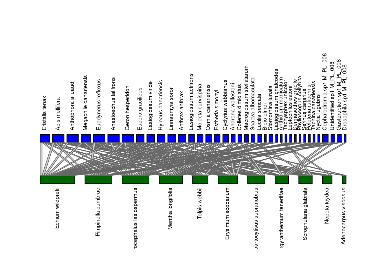
2.2.1 Computing Modularity
Now that we have converted the edge list into a network, we can use the
igraph package to compute modularity. Remember that computing
modularity involves two steps:
- We need to assign each node to a module. We may define modules ourselves(based on a hypothesis or relevant ecological information) or we can run an algorithm to identify modules—using community detection algorithms.
- We then compute the modularity associated to the specified node partition.
Let’s imagine the scenario in which we specify the modules ourselves. We can code modules in the following way:
# Manually define (a random!) partitioning
# We have to assign each node to a module, in this case we have 49 nodes and
# we are (subjectively!) assigning them to 3 modules

node_membership <- c(1,2,2,2,3,2,1,3,2,2,
                     1,2,2,2,3,2,1,3,2,2,
                     1,2,2,2,3,2,1,3,2,2,
                     1,2,2,2,3,2,1,3,2,2,
                     1,2,2,2,3,2,1,3,2)
Now that we have assigned each node to a module, we can visualise this particular node partition:
# Build a color pallete for the modules
colbar <- rainbow(max(node_membership))
# Set the color of each node based on their module
V(M_PL_008_graph)$color <- colbar[node_membership]

# Plot the graph
plot(M_PL_008_graph,
     vertex.label=NA, # if the nodes should be named
     edge.size= 0.2, # the size of the links,
     vertex.size = 5, # the size of the nodes
     layout = layout_nicely)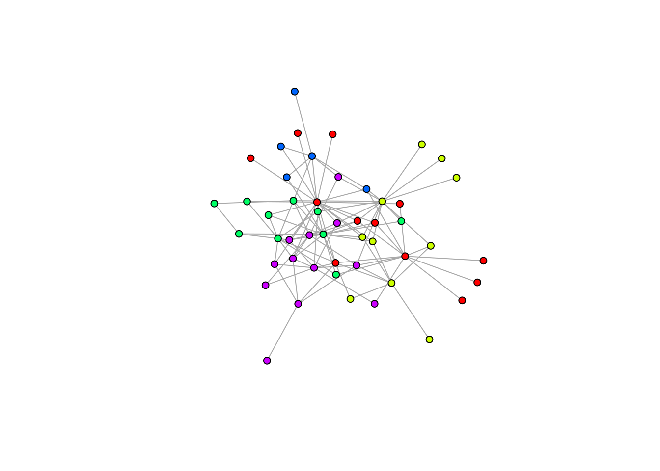
Finally, we can compute the modularity of this node partition using the
modularity function from the igraph package.
## [1] 0.03506586We obtain a very low modularity value, which makes sense since I assigned each node to a module at random.
2.2.2 Finding modules
Instead of partitioning nodes into modules ourselves, we can leverage algorithms that look for partitions that maximise modularity. There are many algorithms to chose from, all with their pros and cons. In most cases you are deciding between accuracy or speed. This may not be a relevant issue if you are working with a network with few nodes, but the computation time can really scale up when working with large networks!
The igraph package includes many algorithms for finding node partitions (also referred to as community detection). Here is a non-exhaustive list:
cluster_edge_betweennesscluster_fast_greedycluster_spinglasscluster_leading_eigencluster_optimal(SLOW!!)
If you’re interested, you can find more about how each algorithm works
by consulting the help file of each function (e.g. ?cluster_optimal).
Let’s go back to our pollination network. Clearly our random partition
was not the best. Let’s use a community detection algorithm to find a
better partition. In this case we will opt for the cluster_fast_greedy
algorithm/function:
# Run the algorithm on our network
modules <- cluster_fast_greedy(M_PL_008_graph)

# We can extract the node membership for the node partition
modules$membership
## [1] 1 2 3 1 5 3 5 4 2 5 3 1 3 1 5 5 5 3 5 2 5 4 2 2 3 3 1 3 5 5 3 2 4 1 1 1 5 2
## [39] 2 2 1 1 1 1 2 5 4 3 4Now we can compute the modularity of the partition found by the algorithm.
# Compute the modularity of this node partition
Q_algorithm <- modularity(M_PL_008_graph, modules$membership)
Q_algorithm
## [1] 0.3428711This gives a much larger modularity value, clearly this partition is better than our random assignment. Finally, we can colour the nodes of our network based on this partition.
# Build a color pallete for the modules
colbar <- rainbow(max(modules$membership))
# Set the color of each node based on their module
V(M_PL_008_graph)$color <- colbar[modules$membership]

# Plot the graph
plot(M_PL_008_graph,
     vertex.label=NA, # if the nodes should be named
     edge.size= 0.2, # the size of the links,
     vertex.size = 5, # the size of the nodes
     layout = layout_nicely)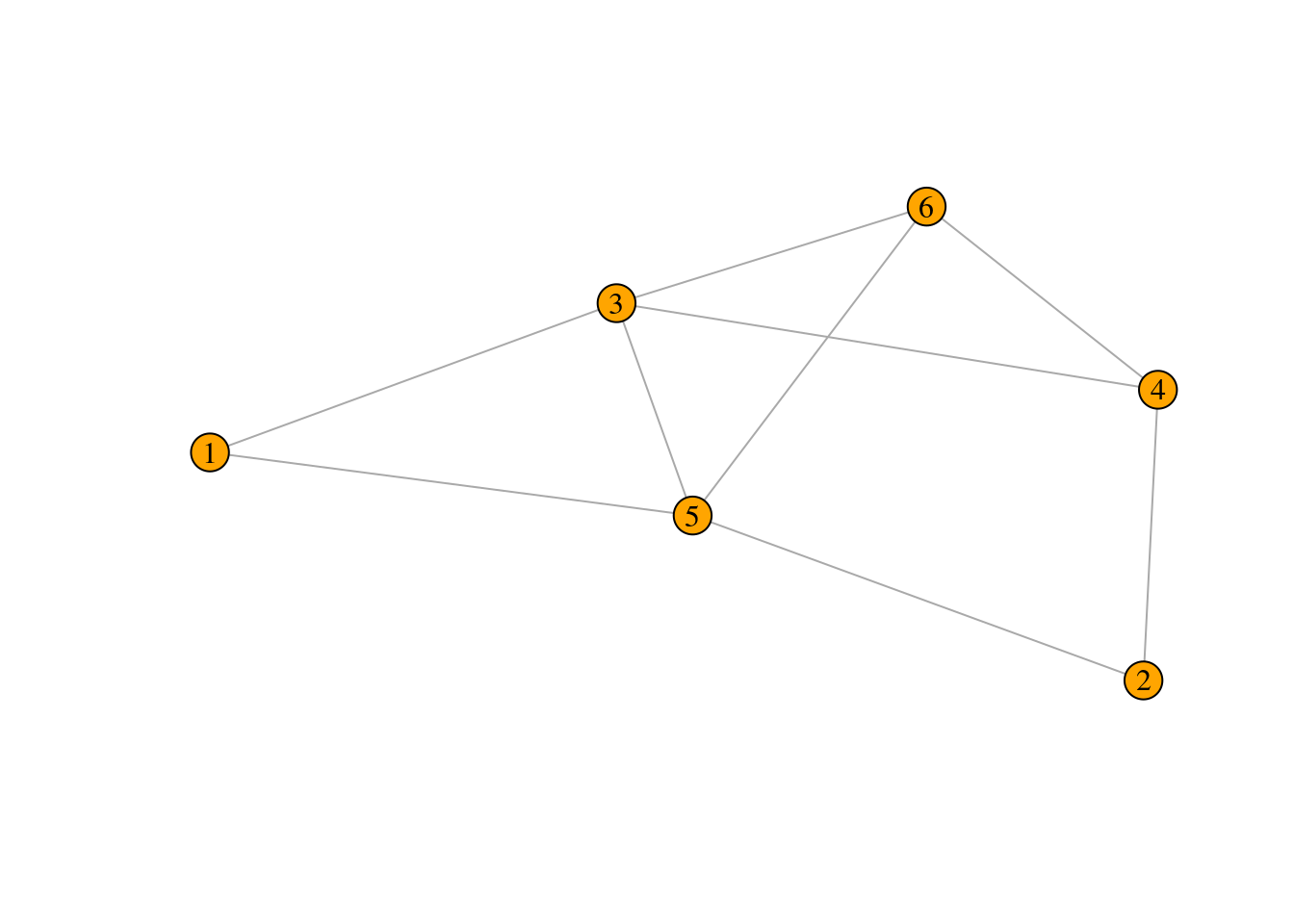
Exercise 4
Now you will replicate the modularity workflow outlined above for the
M_SD_001 network in the Web of Life. Your tasks are the following:
Download the network
M_SD_001using the standard commands.Download the taxonomic information for network
M_SD_001and use this information to assign a type to each node such that the network is made bipartite.Use the community detection algorithm
cluster_louvainto find the optimal node partition for the network.Compute the modularity associated to this node partition.
2.3 Solutions
2.3.1 Exercise 1
For the graph drawn below:
- Write down the degree of each node.
## species 1 species 2 species 3 species 4 species 5 species 6
## 2 2 4 3 4 3- Compute its adjacency matrix.
##      [,1] [,2] [,3] [,4] [,5] [,6]
## [1,]    0    0    1    0    1    0
## [2,]    0    0    0    1    1    0
## [3,]    1    0    0    1    1    1
## [4,]    0    1    1    0    0    1
## [5,]    1    1    1    0    0    1
## [6,]    0    0    1    1    1    0
2.3.2 Exercise 2
Draw the graph represented by the following adjacency matrix:
\[\begin{bmatrix} 0 & 0 & 1 & 0 & 1 \\ 0 & 0 & 0 & 1 & 1 \\ 1 & 0 & 0 & 0 & 0 \\ 0 & 1 & 0 & 0 & 1 \\ 1 & 1 & 0 & 1 & 0 \\ \end{bmatrix}\]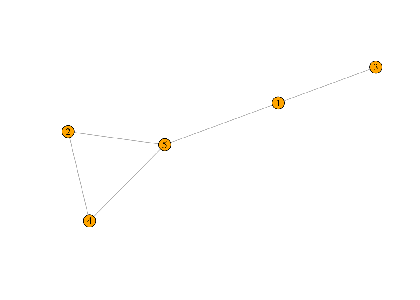
2.3.3 Exercise 3
The node colors of the graph below represent a partitioning of the nodes into three modules.
- Use the formula given in the Food Webs lecture to compute the modularity associated with the partition.
## [1] "modularity: 0.2734375"- Do you think the given node partitioning is the best, i.e. it optimizes modularity (argue)?
# The modularity of the network will be higher if nodes 1 to 4 all belong to the
# same module as can be seen below:

# Redefine modules
membership_for_modularity <- c(1,1,1,1,2,2,2)
my_modularity <- modularity(graph, membership_for_modularity)
print(paste("new modularity:",my_modularity))
## [1] "new modularity: 0.3671875"2.3.4 Exercise 4
- Download the network
M_SD_001using the standard commands.
# Download the M_SD_001 network from the web-of-life
json_url <- paste0("https://www.web-of-life.es/get_networks.php?network_name=M_SD_001")
my_edge_data <- jsonlite::fromJSON(json_url)

# Keep only the three relevant columns and use them to create the network
my_network <- my_edge_data |>
  dplyr::select(species1, species2, connection_strength) |>
  # convert the connection_strength column to numeric
  mutate(connection_strength = as.numeric(connection_strength)) |>
  graph_from_data_frame(directed = FALSE)

# Get a glimpse of the network
my_network
## IGRAPH a8d07fa UN-- 28 50 --
## + attr: name (v/c), connection_strength (e/n)
## + edges from a8d07fa (vertex names):
## [1] Celastrus orbiculatus--Euphagus carolinus
## [2] Cornus florida --Cardinalis cardinalis
## [3] Celastrus orbiculatus--Cardinalis cardinalis
## [4] Lindera benzoin --Cardinalis cardinalis
## [5] Smilax rotundifolia --Cardinalis cardinalis
## [6] Lonicera japonica --Cardinalis cardinalis
## [7] Vitis sp1 M_SD_001 --Cardinalis cardinalis
## [8] Rhus radicans --Parus atricapillus
## + ... omitted several edges- Download the taxonomic information for network
M_SD_001and use this information to assign a type to each node such that the network is made bipartite.
# Download taxonomic data from the Web of Life for our downloaded network
# In this case we specify network_name=M_SD_001
my_taxonomic_data <- read.csv(
  paste0("https://www.web-of-life.es/","get_species_info.php?network_name=M_SD_001"))

# First reorder the taxonomic data so that it follows the
# same order of species as the network we created
my_taxonomic_data <- my_taxonomic_data[match(names(V(my_network)),
                                             my_taxonomic_data$species), ]

# Extract the information from the is.resource column
isResource <- as.logical(my_taxonomic_data$is.resource) # convert data to T/F

# Add the "type" attribute to the nodes of the graph
V(my_network)$type <- !(isResource)

# Check if network is bipartite
is_bipartite(my_network)
## [1] TRUE- Use the community detection algorithm
cluster_louvainto find the optimal node partition for the network.
# Run the algorithm on our network
my_modules <- cluster_louvain(my_network)

# We can extract the node membership for the node partition
my_modules$membership
## [1] 1 2 3 1 1 4 5 1 1 5 3 2 4 1 1 3 1 1 3 4 2 5 1 5 5 4 2 5- Compute the modularity associated to this node partition.
# Compute the modularity of this node partition
Q_my_network <- modularity(my_network, my_modules$membership)
Q_my_network
## [1] 0.2898- EXTRA STEP (not evaluated!) I plot the network and colour nodes by the module they belong to.
# Build a color pallete for the modules
colbar <- rainbow(max(my_modules$membership))
# Set the color of each node based on their module
V(my_network)$color <- colbar[my_modules$membership]

# Plot the graph
plot(my_network,
     vertex.label=NA, # if the nodes should be named
     edge.size= 0.2, # the size of the links,
     vertex.size = 5, # the size of the nodes
     layout = layout_nicely)