Chapter 5 Null models
Fernando Pedraza
session 20/03/2025
In this session, we will cover how to use null models to provide randomisations of matrices representing ecological networks. First, you perform randomisations “by hand” using the null models covered in the morning lecture. Then, you will learn the necessary commands to replicate the analyses in R. We will continue working with networks from the Web of Life, so we will reuse some concepts and commands from the previous sessions (Toolkit for network analysis).
5.1 Null models by hand
In this section you will randomize networks “by hand” following the null
models covered during the morning lecture. Some null models will require
you to generate random numbers and perform simple arithmetic operations.
Feel free to use R for these purposes (hint: use the runif() function
to generate random numbers).
Exercise 1
Consider a network represented by the following adjacency matrix:
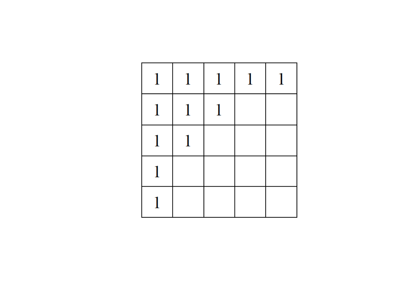
Provide a randomization of the matrix using:
The Equifrequent Null Model
The Probabilistic Cell Null Model
Please solve this exercise on a piece of paper. When you have finished, take a picture of your solution and upload it (along with the rest of your submission) into the corresponding folder on OLAT.
Exercise 2
Consider a network represented by the following adjacency matrix:
Provide three iterations of the Swap Null Model.
Please solve this exercise on a piece of paper. When you have finished, take a picture of your solution and upload it (along with the rest of your submission) into the corresponding folder on OLAT.
5.2 Computer part I
In this section we will use R code to run the null models covered during this morning’s lecture. We will focus on using the null models to evaluate the statistical significance of the nestedness value of a single network. Ultimately, we want to know if the measured nestedness value of our network is significantly different from the nestedness values obtained from a set of random iterations.
To do this, we will first define a network and compute its nestedness. Then, we’ll compute nestedness again using three null models. Finally, we will estimate the significance of the nestedness value using the z-score.
To start, we load the packages we will use for this session. Please note
that we will use the rweboflife package to run the null models and
compute nestedness.
# Load packages
library(igraph)
library(dplyr)
library(bipartite)
library(rweboflife)

# To install the rweboflife package, uncomment the following line and run it:
#devtools::install_github("bascompte-lab/rweboflife", force = TRUE)
5.2.1 Dowloading a network and computing its nestedness
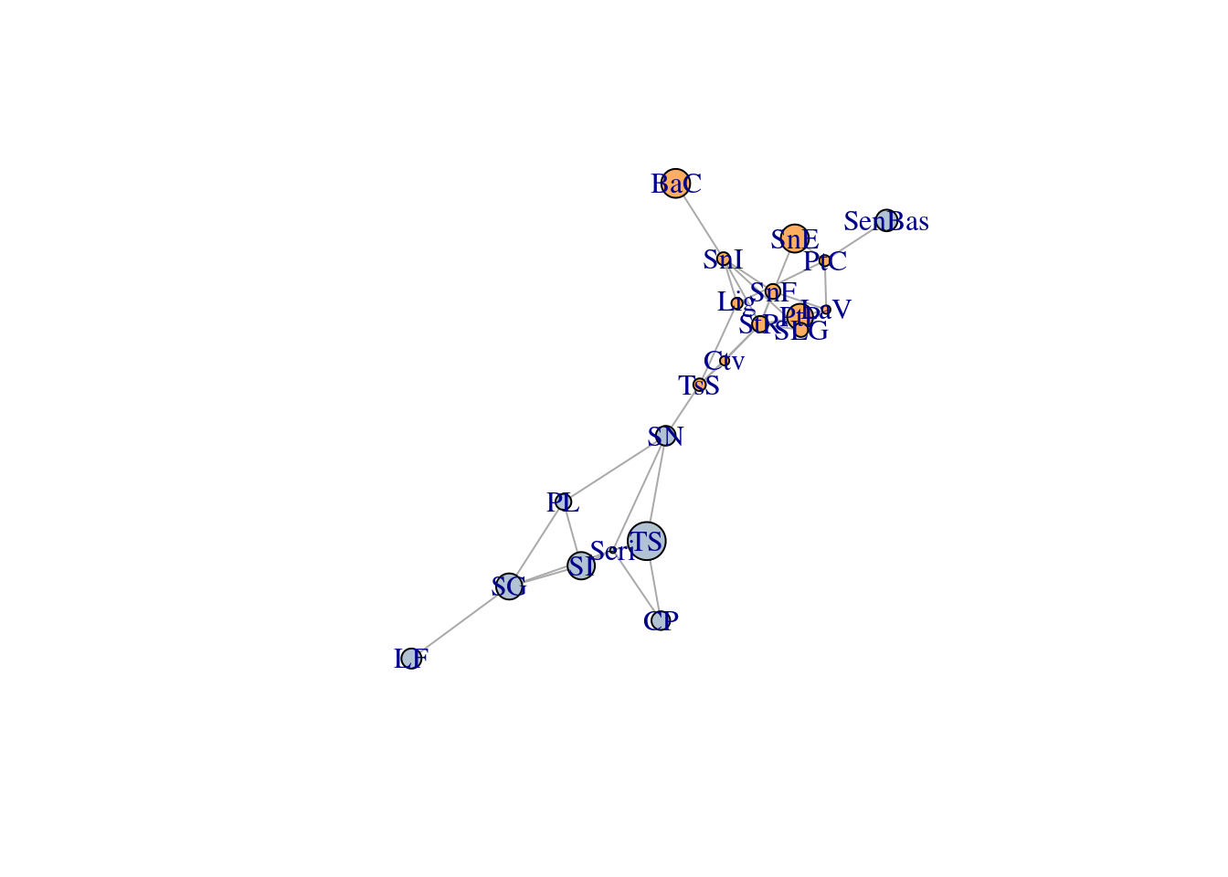
We will evaluate the significance of the nestedness value of a
pollination network from the Web of Life (M_PL_036). We first download
the network and visualise it:
# Define the url associated with the network to be downloaded
json_url <- "https://www.web-of-life.es/get_networks.php?network_name=M_PL_036"

# Download the network (as a dataframe)
network_data <- jsonlite::fromJSON(json_url)

# Keep only the three relevant columns and use them to create the network
network <- network_data |>
  dplyr::select(species1, species2, connection_strength) |>
  # convert the connection_strength column to numeric
  dplyr::mutate(connection_strength = as.numeric(connection_strength)) |>
  graph_from_data_frame(directed = FALSE)

# Convert the network into bipartite format
V(network)$type <- bipartite.mapping(network)$type

# Assign different colours to plants and pollinators
V(network)$color <- ifelse(V(network)$type == TRUE, "blue", "orange")

# Plot network using bipartite layout
plot(network,
     layout=layout_as_bipartite,
     arrow.mode=0,
     vertex.label=NA,
     vertex.size=4,
     asp=0.2)
Next we compute its nestedness value (as demonstrated in the previous session):
# Convert the igraph bipartite network into an incidence matrix
network_matrix <- as_incidence_matrix(network, sparse=FALSE)

# Compute network nestedness
observed_nestedness <- rweboflife::nestedness(network_matrix)

# Print value
observed_nestedness
## [1] 0.4136637We conclude that the network has a nestedness value of 0.41. But is this value statistically meaningful?
To answer this question, we can leverage null models. More specifically, we can use a null model to generate randomisations of our network. Once it has been randomised, we can compute the nestedness value of the random matrix. With enough randomisations, we will be able to compare our observed nestedness value with the distributions of nestedness values arising from the randomised matrices. To determine the statistical significance of the observed nestedness value, we can use z-score test.
The function null_model from the rweboflife package allows you to
run the equifrequent null model, probabilistic cell null model, and the
swap null model. This function takes three arguments:
M_inspecifies the matrix you wish to randomisemodelspecifies the null model you wish to use to randomise the matrix (you can choose from:"equifrequent","cell"and"swap")iter_maxdetermines how many iterations to run. Note that this parameter is only relevant when running the swap algorithm.
Next, I demonstrate the procedure of evaluating the significance of the
observed nestedness value of M_PL_036 using the equifrequent null
model.
5.2.2 Equifrequent null model
As mentioned above, we will use the null_model function from the
rweboflife package to implement the equifrequent null model. To run
the equifrequent model on the network we previously defined, we run the
following command:
randomistion_equifrequent <-  rweboflife::null_model(M_in = network_matrix,
                                                        model = "equifrequent",
                                                        iter_max = 1)
The object randomistion_equifrequent is storing a matrix that has been
randomised using the equifrequent null model:
##       [,1] [,2] [,3] [,4] [,5] [,6] [,7] [,8] [,9] [,10] [,11] [,12]
##  [1,]    0    0    0    1    0    1    0    0    1     1     0     1
##  [2,]    0    0    0    0    0    1    0    0    0     0     0     0
##  [3,]    0    0    0    0    0    0    0    0    0     0     0     1
##  [4,]    0    0    0    0    0    0    0    0    0     0     1     0
##  [5,]    0    0    1    0    0    0    1    0    0     1     1     0
##  [6,]    0    0    1    0    1    0    0    0    1     1     0     0
##  [7,]    0    1    1    1    0    0    0    0    0     1     0     0
##  [8,]    0    0    1    0    0    0    0    0    1     0     0     1
##  [9,]    0    0    0    0    0    0    0    0    1     0     1     1
## [10,]    0    0    1    0    0    0    0    0    1     0     1     1
We now can compute the nestednesss value of the randomised matrix:
# Calculate the nestedness value for our network and store it
nestedness_randomistion_equifrequent <- rweboflife::nestedness(
                                          randomistion_equifrequent)
nestedness_randomistion_equifrequent
## [1] 0.3337838The observed nestedness value differs between the empirical network and its randomisation. However, a single randomisation is not enough to draw a conclusion. Instead, we should perform several randomistations and compute the nestedness value of each one. Then, we can compare the nestedness value of the empirical network with the distribution of nestedness values from our randomisations. Let’s generate 50 randomisations of our network and compute nestedness for each one.
# define number of randomisations
n <- 50

# Run the null model n times and compute the nestedness value of each randomised
# matrix
nestedness_from_equifrequent <- replicate(n, {
  rweboflife::nestedness(
    rweboflife::null_model(M_in = network_matrix,
                           model = "equifrequent",
                           iter_max = 1)
  )
})

# Print out resulting nestedness values
nestedness_from_equifrequent
## [1] 0.2462462 0.3447447 0.2651652 0.3370871 0.3121622 0.3046547 0.2539039
## [8] 0.3783784 0.3319820 0.3126126 0.2620120 0.3166667 0.3109610 0.2567568
## [15] 0.3010511 0.3070571 0.2650150 0.3235736 0.3489489 0.2507508 0.2927928
## [22] 0.3683183 0.3114114 0.3235736 0.3009009 0.2229730 0.2567568 0.2941441
## [29] 0.3112613 0.3641141 0.2515015 0.2867868 0.3475976 0.2671171 0.3675676
## [36] 0.3567568 0.2629129 0.2912913 0.2530030 0.2963964 0.3223724 0.3235736
## [43] 0.3253754 0.3054054 0.3777778 0.3563063 0.2855856 0.3306306 0.3543544
## [50] 0.4018018Now that we have our nestedness estimates, we need to estimate the significance of the nested value we initially observed using the z-score. The formula to estimate z-scores is:
\[ z-score = \frac{observed\ nestedness - mean(nestedness)}{sd(nestedness)} \]
To calculate the z-score, we first have to obtain the mean and the
standard deviation of the nestedness values we obtain from our null
model. The mean and standard deviation are calculated in R with the
mean and sd functions, respectively.
# Compute mean for nestedness values estimated by null model
mean_nestedness <- mean(nestedness_from_equifrequent)
# Compute sd for nestedness values estimated by null model
sd_nestedness <- sd(nestedness_from_equifrequent)
Now we can calculate the z-score for the null model.
# Compute z score following formula
z_score <- (observed_nestedness - mean_nestedness)/sd_nestedness
Finally we can calculate the probability associated to the z-score using
the pnorm and setting the lower.tail parameter to FALSE.
# Compute associated p value
p_val_equi <-pnorm(z_score, lower.tail = FALSE)

# Print p value
print(p_val_equi)
## [1] 0.005615611We obtain a low p-value (\(<0.05\)), this suggests that the observed nestedness value is significantly different from the nestendess values of the randomised matrices. In other words, the observed network is more nested than what we would expect to see by chance.
Exercise 3
Determine the significance of the nestedness value of M_PL_036 using
the probabilistic cell null model. You should do the following:
- Run the null model 50 times using the
null_modelfunction. - Compute the mean and standard deviation of our null model estimates.
- Calculate the z-score.
- Obtain an associated p-value.
Exercise 4
Determine the significance of the nestedness value of M_PL_036 using
the swap null model. You should do the following:
- Run the null model 50 times with using the
null_modelfunction. Note that this time you should use theiter_maxparameter to specify that the null model should perform 20 iterations. - Compute the mean and standard deviation of our null model estimates.
- Calculate the z-score.
- Obtain an associated p-value.
5.3 Computer part II
In this final section we will use null models to test whether a set of pollination networks are significantly more or less nested than a set of seed dispersal networks.
5.3.1 Code
To save some time, I have already downloaded the necessary networks. The
first thing we need to is to load the networks. The seed dispersal
networks are stored as entries in the list called seed_networks which
is found in the seed_networks.Rdata file. The pollination networks are
stored as entries in the list called pollination_networks which is
found in the pollination_networks.Rdata file. We will begin by loading
these two files.
# Load pollination networks
load("~/ecological_networks_2025/downloads/Data/null_models/pollination_networks.Rdata")

# Load seed networks
load("~/ecological_networks_2025/downloads/Data/null_models/seed_networks.Rdata")

# Note that the load function directly creates an R object where the data is
# read into(!). In this case, after running the commands, you should have
# two new objects in your environment: seed_networks and pollination_networks.
Now that we have our networks, we can run the null models. For this exercise, we will use the cell null model. Let’s outline our workflow:
- First, compute the nestedness value of each of the networks in the
seed_networksandpollination_networkslists. - Next, perform 10 randomisations of each network using the cell null model.
- Finally, run a t-test to determine whether there are differences between the two types of networks in relation to their standardized nestedness values.
Below you will find the code to perform the workflow outlined above. However, if you’re up for a challenge, feel free to write your own code. Use the p-value you obtain to answer the question at the bottom of this section.
#################################################
# SEED DISPERSER NETWORKS
#################################################

# calculate nestedness value of each empirical network
seed_nestedness <- sapply(seed_networks,
                          rweboflife::nestedness)

# generate 10 randomisations of each seed dispersal network using the equifrequent model
seed_randomisations <- replicate(10, lapply(seed_networks,
                          rweboflife::null_model,  model = 'cell' ))

# compute the nestedness value of each randomisation
seed_randomisations_nestedness <- sapply(t(seed_randomisations),
                                         rweboflife::nestedness)

# extract nestedness value of each randomisation
seed_randomisations_nestedness <- split(seed_randomisations_nestedness,
      ceiling(seq_along(seed_randomisations_nestedness)/10))

# compute mean nestedness of each randomisation
mean_seed_randomisations_nestedness <- sapply(
  seed_randomisations_nestedness, mean)

# compute sd nestedness of each randomisation
sd_seed_randomisations_nestedness <- sapply(
  seed_randomisations_nestedness, sd)

# calculate z-score of each network
seed_z_score <-
  (seed_nestedness - mean_seed_randomisations_nestedness)/
  sd_seed_randomisations_nestedness

#################################################
# POLLINATION NETWORKS
#################################################

# calculate nestedness value of each empirical networks
pollination_nestedness <- sapply(pollination_networks,
                                 rweboflife::nestedness)

# generate 10 randomisations of each seed dispersal network using the equifrequent model
pollination_randomisations <- replicate(10, lapply(pollination_networks,
                                                   rweboflife::null_model,
                                                   model = 'cell'))

# compute the nestedness value of each randomisation
pollination_randomisations_nestedness <- sapply(
  t(pollination_randomisations), rweboflife::nestedness)

# extract nestedness value of each randomisation
pollination_randomisations_nestedness <- split(pollination_randomisations_nestedness,
 ceiling(seq_along(pollination_randomisations_nestedness)/10))

# compute mean nestedness of each randomisation
mean_pollination_randomisations_nestedness <- sapply(pollination_randomisations_nestedness,
                                                     mean)

# compute sd nestedness of each randomisation
sd_pollination_randomisations_nestedness <- sapply(pollination_randomisations_nestedness,
                                                   sd)

# calculate z-score of each network
pollination_z_score <- (pollination_nestedness -
                          mean_pollination_randomisations_nestedness)/
  sd_pollination_randomisations_nestedness

# Use a t.test to determine whether there are significant differences in the
# nestedness values of the pollination and seed dispersal networks
t.test(seed_z_score, pollination_z_score)
Exercise 6
Run the workflow outlined above and take a look at the output of the t-test. Are there differences in the nestedness of the networks? How do your findings compare to the findings described in Figure 2 of Bascompte et al. 20031?
Solutions
Please note that I will not provide solutions for Exercises 1 and 2 since my randomisations will likely differ from yours.
Exercise 3
Determine the significance of the nestedness value of M_PL_036 using
the probabilistic cell null model. You should do the following:
- Run the null model 50 times using the
null_modelfunction. - Compute the mean and standard deviation of our null model estimates.
- Calculate the z-score.
- Obtain an associated p-value.
### CELL  ###

# Run the null model n times and compute the nestedness value of each randomised
# matrix
nestedness_from_cell <- replicate(50, {
  rweboflife::nestedness(
    rweboflife::null_model(M_in = network_matrix,
                           model = "cell",
                           iter_max = 1)
  )
})

# Compute mean for nestedness values estimated by null model
mean_nestedness <- mean(nestedness_from_cell)
# Compute sd for nestedness values estimated by null model
sd_nestedness <- sd(nestedness_from_cell)

# Compute z score following formula
z_score <- (observed_nestedness - mean_nestedness)/sd_nestedness


# Compute associated p value
p_val_cell <-pnorm(z_score, lower.tail = FALSE)## [1] 0.2254491Exercise 4
Determine the significance of the nestedness value of M_PL_036 using
the swap null model. You should do the following:
- Run the null model 50 times with using the
null_modelfunction. Note that this time you should use theiter_maxparameter to specify that the null model should perform 20 iterations. - Compute the mean and standard deviation of our null model estimates.
- Calculate the z-score.
- Obtain an associated p-value.
### SWAP ###

# Run the null model n times and compute the nestedness value of each randomised
# matrix
nestedness_from_swap <- replicate(50, {
  rweboflife::nestedness(
    rweboflife::null_model(M_in = network_matrix,
                           model = "swap",
                           iter_max = 20)
  )
})

# Compute mean for nestedness values estimated by null model
mean_nestedness <- mean(nestedness_from_swap)
# Compute sd for nestedness values estimated by null model
sd_nestedness <- sd(nestedness_from_swap)

# Compute z score following formula
z_score <- (observed_nestedness - mean_nestedness)/sd_nestedness

# Compute associated p value
p_val_swap <-pnorm(z_score, lower.tail = FALSE)## [1] 0.007579373Exercise 5
Compare the conclusions about the significance of nestedness across the three null models. In your Rscript, discuss any differences you may have obtained.
Our p-values are the following:
## [1] 0.005615611## [1] 0.2254491## [1] 0.007579373There is a large difference in the p-values obtained from the null models. The p-values obtained from the equifrequent and swap null model suggest that the observed nestedness value is statistically meaningful (p < 0.05). However, the p-value obtained from the cell null model suggest a nestedness value that is not significant (!). Note that the p-values you obtain will likely differ from mine, because running the null model algorithms multiple times will give slightly different randomised matrices.
The important thing to take from this exercise is that your choice of a null model can affect your conclusions. Thus, is important to be aware of the strengths and weaknesses of each null model and choose wisely.
Exercise 6
Run the workflow outlined above and take a look at the output of the t-test. Are there differences in the nestedness of the networks? How do your findings compare to the findings described in Figure 2 of Bascompte et al. 2003?
The output of the t-test should look something like this:
##  Welch Two Sample t-test

##

## data:  seed_z_score and pollination_z_score

## t = -0.7027, df = 17.625, p-value = 0.4914

## alternative hypothesis: true difference in means is not equal to 0

## 95 percent confidence interval:

##  -1.4311341  0.7145558

## sample estimates:

## mean of x mean of y

## 0.6255704 0.9838595
From the t-test we can conclude that there are no significant differences in the nestedness values of pollination and seed dispersal networks (p = 0.49). This result is in agreement with the findings described Figure 2 of Bascompte et al. 2003.
Bascompte, J., Jordano, P., Melián, C.J. and Olesen, J.M. The nested assembly of plant-animal mutualistic networks. PNAS 100(16), 9383-9387 (2003).↩︎