Chapter 7 Measuring network robustness

Fernando Gonçalves
session 26/03/2025

In the morning lecture we studied together the topological robustness of networks, possible ways to quantify it and what are the properties of networks that can affect their robustness. Here, we will simulate the extinction of species in two different networks and measure how robust these networks are to different types of extinctions. We will measure the topological robustness of these networks looking into how the size of the largest component in them changes as we progressively remove species. In networks, a component is a set of nodes that are completely isolated from other nodes in the network. Most real-world networks contain most of its nodes in a single component, called a giant component. Understanding the processes that causes the loss of this giant component and breaks networks into multiple components is one of the major goals of the field of percolation theory in statistical physics. For ecological networks, the loss of a giant component implies a significant loss of interactions and, therefore, of function in an ecological community.

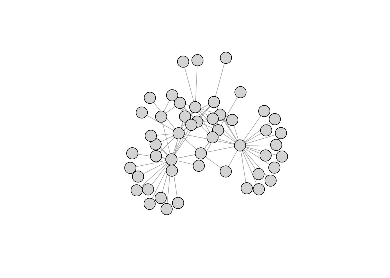
For this exercise section we will use two networks. One with low values of nestedness, and another one with high values of nestedness. First, let`s import and plot these networks so we can visualize their topology.

7.1 Load data

# Import igraph package
library(igraph)

# Read networks
n1<-graph_from_incidence_matrix(read.csv(file="~/ecological_networks_2025/downloads/Data/measuring_networks_robustness/network_nested_low.csv", header=F))
n2<-graph_from_incidence_matrix(read.csv(file="~/ecological_networks_2025/downloads/Data/measuring_networks_robustness/network_nested_high.csv", header=F))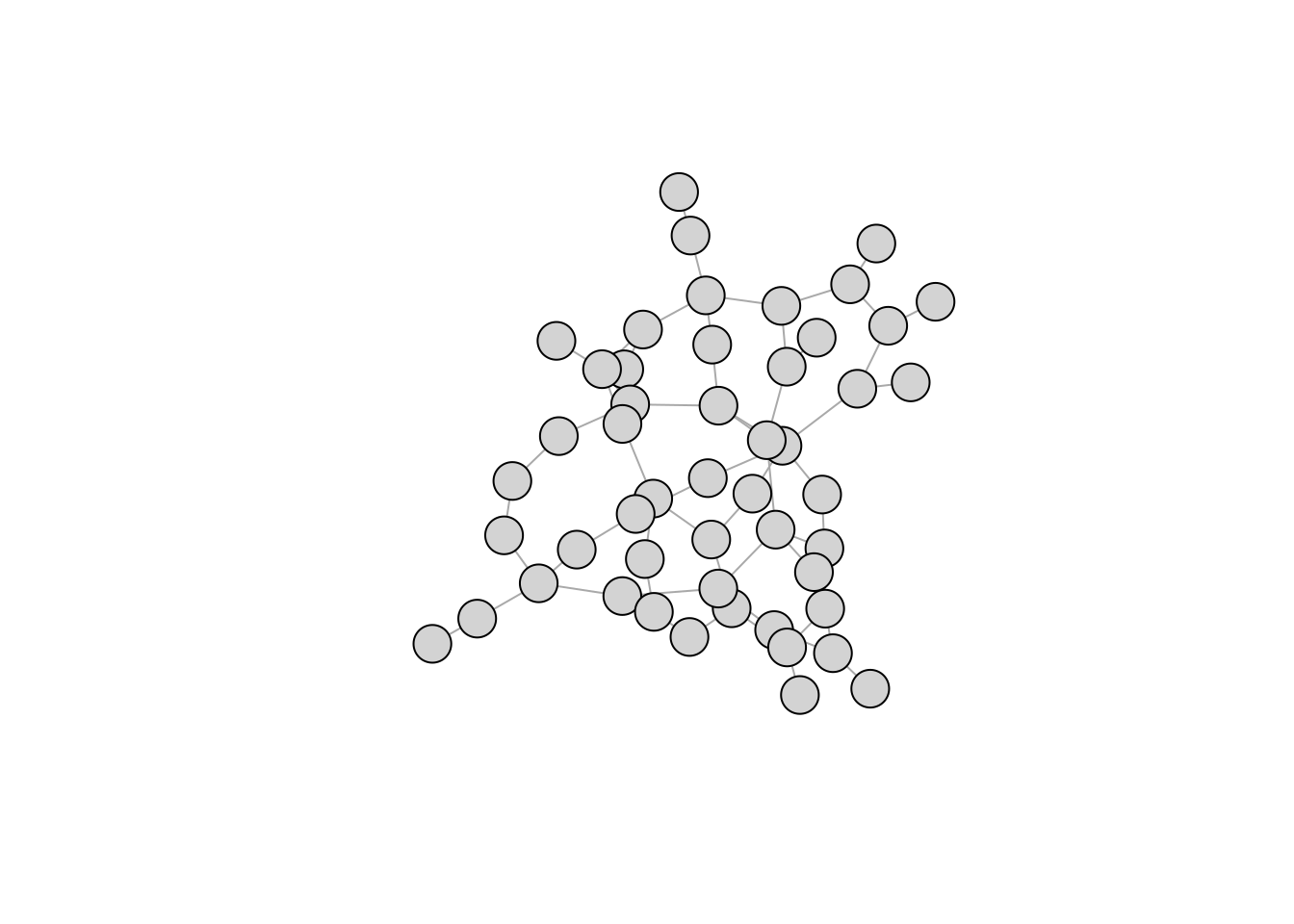

plot(n1, vertex.label=NA, vertex.color="lightgray")

plot(n2, vertex.label=NA, vertex.color="lightgray")

7.2 Random extinctions

As we can see, both of these networks contain a single, giant component. Our next step will be to write a function that progressively remove species in the network and keeps track of the size of the largest component. In this first part of the exercise section, we will write a function that progressively remove species at random. Later, we will look into targeted extinctions, in which we preferentially target certain species in the network. The first function, reproduced below, perform the following steps:

Randomly select a species in the network.
Remove this species from the network.
Measure the size of the largest component in the network after this extinction.
Repeat the above three steps until there is only one species left in the network.

random_extinctions<-function(network){
  
  #Setting up the data structure to store the results
  
  #Vector for storing the size of the largest component 
  # in the network after each species extinction
  size_comp<-c() 
  #Vector to store the cumulative number of extinctions in the network
  n_extinct<-c()
  #Variable identifying the steps of the loop of extinction
  i<-0 
  #Retrieving the initial number of species in the network
  n_nodes<-length(V(network))
  
  #Simulating the progressive extinction of species
  
  while(n_nodes > 1){
    
    # Step (1)
    id<-sample(1:n_nodes, 1) 
    #Step (2)
    network<-delete_vertices(network, id) 
    #Updating the variable 
    i<-i+1 
    #Storing the cumulative number of extinct species
    n_extinct[i]<-i 
    #Step (3)
    size_comp[i]<-max(igraph::components(network)$csize) 
    #Updating the number of species in the network after extinction
    n_nodes<-length(V(network)) 
    
  }
  
  return(data.frame(n_extinct, size_comp))
  
}

With this function, we can now look into how our two different networks respond to the progressive random extinction of species. Since this is a stochastic function, we will perform 20 replicates of these random extinctions for each network and look into the average results.

#Performing 20 replicates for the low nestedness network
net1_random<-do.call(rbind, 
                     replicate(n=20, random_extinctions(n1), simplify=FALSE)) 

#Computing the average results of the 20 replicates
net1_random<-aggregate(.~n_extinct, FUN=mean, data=net1_random) 

#Identifying the results of this network as the "Low nestedness" one.
net1_random$Nestedness<-"Low nestedness" 

#Performing 20 replicates for the high nestedness network
net2_random<-do.call(rbind, 
                     replicate(n=20, random_extinctions(n2), simplify=FALSE)) 

#Computing the average results of the 20 replicates
net2_random<-aggregate(.~n_extinct, FUN=mean, data=net2_random) 

#Identifying the results of this network as the "High nestedness" one.
net2_random$Nestedness<-"High nestedness"

# Setting up a single data frame containing the results for both networks
results_random<-rbind(net1_random, net2_random) 

#Plotting the results
library(ggplot2)

ggplot(data = results_random, aes(x = n_extinct, y=size_comp, color=Nestedness)) +
  geom_line(size=1) +
  ylab("Size of the largest component") + xlab("Number of extinctions") +
  theme_bw() +
  theme(panel.grid=element_blank())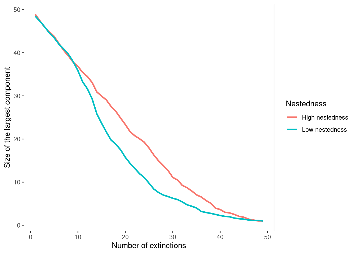

7.2.1 Exercise: Random extinctions

Questions

With the results depicted by the figure above, answer the following questions:

What differences can you observe in how the size of the largest component changes with extinctions in the two networks?
Which network is more likely to fragment into multiple components under a progressively loss of species at random?

7.3 Non-random extinctions

For this second part of the exercise section we will now simulate extinctions when some species are preferentially targeted. To do so, we will modify the previous function so that species get extinct in a particular order, instead of randomly. Here, we will sequentially remove species from the network starting with the one that interact with the most species, i.e., the one with the highest degree, to the ones with the lowest degree. Therefore, we will simulate networks in which generalist species get extinct first. The modified function is reproduced below:

target_extinctions<-function(network){
  
  #Setting up the data structure to store the results
  
  #Vector for storing the size of the largest component 
  # in the network after each node extinction
  size_comp<-c()
  #Variable to store the cumulative number of extinctions in the network
  n_extinct<-c()
  #Variable identifying the loop
  i<-0 
  n_nodes<-length(V(network))
  
  while(n_nodes > 1){
    #Sorting species from high to low degree and getting their index
    id<-sort(igraph::degree(network), decreasing=TRUE, index.return=T)$ix 
    #Deleting the one with the highest degree (position 1 in the sorted vector)
    network<-delete_vertices(network, id[1]) 
    i<-i+1
    n_extinct[i]<-i
    size_comp[i]<-max(igraph::components(network)$csize)
    n_nodes<-length(V(network))
    
  }
  
  return(data.frame(n_extinct, size_comp))
  
}

With this function, we can now verify the topological robustness of the low and high nestedness networks to targeted extinctions. Since these extinctions follow a particular order and are deterministic, we do not need several replicates.

7.3.1 Exercise: Non-random extinctions

Use the target_extinctions function to simulate the targeted node removal for the low and high nestedness networks. Produce a plot to visualize the change in the size of the largest components and the differences among the networks.

Questions

With the figure you produce, answer the following questions:

What differences can you observe in how the size of the largest component changes with extinctions from the random to the targeted scenarios?
Which network is more topologically robust to the loss of generalist species? Try to come up with a hypothesis to explain your answer.

7.4 Solutions

7.4.1 Exercise: Random extinctions

Questions

With the results depicted by the figure above, answer the following questions:

What differences can you observe in how the size of the largest component changes with extinctions in the two networks?

Answer: In the highly nested network, the size of the largest component decreases approximately linearly as extinctions increase. In contrast, the less nested network initially follows a similar linear decline, but once the largest component shrinks to a tipping point (around 38) its size begins to decrease more rapidly compared to the highly nested network.

Which network is more likely to fragment into multiple components under a progressively loss of species at random?

Answer: The network with low nestedness is more prone to fragmenting into multiple disconnected components under random species loss. This is because its largest component declines more rapidly as extinctions increase, indicating a higher likelihood of fragmentation.

7.4.2 Exercise: Non-random extinctions

#Simulating targeted extinctions in the low nestedness network
net1_target<-target_extinctions(n1); net1_target$Nestedness<-"Low nestedness"
#Simulating targeted extinctions in the low nestedness network
net2_target<-target_extinctions(n2); net2_target$Nestedness<-"High nestedness"
# Merging the results of the two networks together
results_target<-rbind(net1_target, net2_target)

#Creating a variable to identify the random scenario
results_random$Scenario<-"Random"
#Creating a variable to identify the targeted scenario
results_target$Scenario<-"Targeted"
#Merging the results of all scenarios together in a data frame
all_results<-rbind(results_random, results_target)


ggplot(data=all_results,
       aes(x=n_extinct, y=size_comp, color=Nestedness, linetype=Scenario))+
  geom_line(size=1)+
  ylab("Size of the largest component")+xlab("Number of extinctions")+
  theme_bw()+
  theme(panel.grid=element_blank())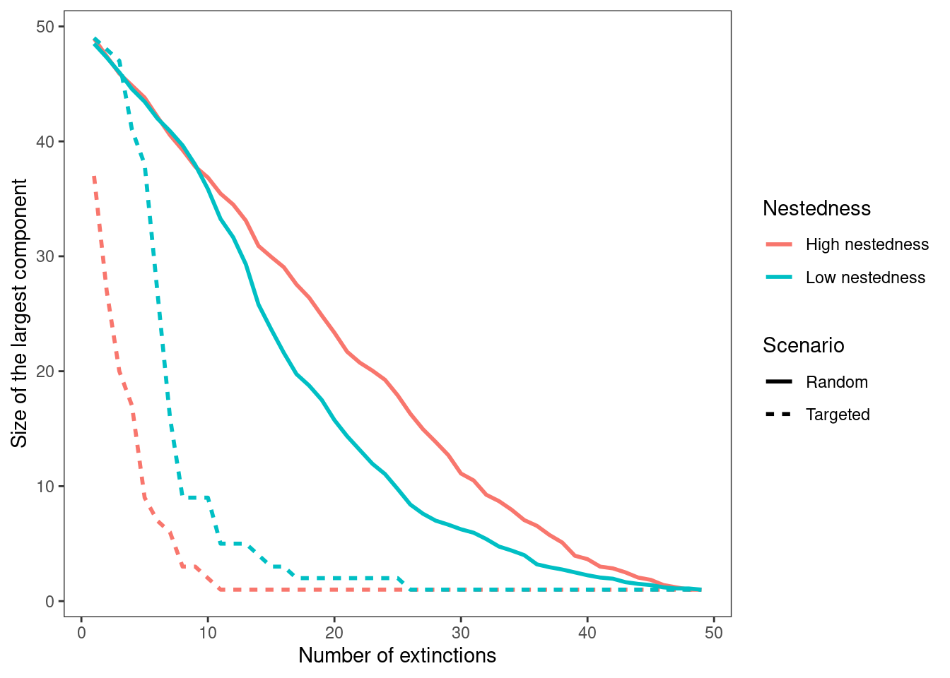

Questions

With the figure you produce, answer the following questions:

What differences can you observe in how the size of the largest component changes with extinctions from the random to the targeted scenarios?

Answer: The size of the largest component declines significantly faster in targeted extinction scenarios compared to random extinctions. In highly nested networks, this decline is even more pronounced, as the largest component shrinks more rapidly with increasing extinctions compared to networks with lower nestedness. This suggests that highly nested structures are more vulnerable to targeted disruptions, leading to a quicker breakdown of connectivity within the network.

Which network is more topologically robust to the loss of generalist species? Try to come up with a hypothesis to explain your answer.

Answer: The network with lower nestedness is more topologically robust to the loss of generalist species. While both networks collapse rapidly, the low-nestedness network retains a larger connected component for a slightly longer period. A possible explanation is that in low- nestedness networks, interactions are more evenly distributed among species. This reduces the cascading effects of removing a single node, unlike in highly nested networks, where many specialist species rely on a few highly connected generalists, making the structure more vulnerable to their loss.