Chapter 4 Measuring nestedness
Leandro Cosmo
session 19/03/2025
In this session, we will cover how to measure the nestedness of an ecological network. First, you will quantify connectance and nestedness “by hand” (with help from these slides) and then you will learn the necessary commands to replicate the analysis in R. We will continue working with networks from the Web of Life, so we will reuse some concepts and commands from the previous sessions (Toolkit for network analysis).
4.1 Introduction
Nestedness is a measure of the structure of bipartite networks. Ecological networks, such as plant-pollinator networks, are often nested.
There are many different measures of nestedness. We will focus on a modified version of the NODF measure (Almeida-Neto et al., 2008) which was used, for example, in Fortuna et al. (2019) to investigate networks of bacteria and phages.
Almeida-Neto, M., Guimarães, P., Guimarães, P.R., Ulrich, W.: A consistent metric for nestedness analysis in ecological systems: reconciling concept and measurement. Oikos, 1227–1239 (2008). DOI 10.1111/j.2008.0030-1299.16644.xh
Fortuna, M.A., Barbour, M.A., Zaman, L., Hall, A.R., Buckling, A. and Bascompte, J.: Coevolutionary dynamics shape the structure of bacteria‐phage infection networks. Evolution 1001-1011 (2019). DOI 10.1111/evo.13731
4.2 Nestedness by hand
We begin with a quick warm-up for constructing networks and measuring their connectance and nestedness.
Exercise 1
For the bipartite graph drawn below:
- write down the incidence matrix B
- compute connectance C
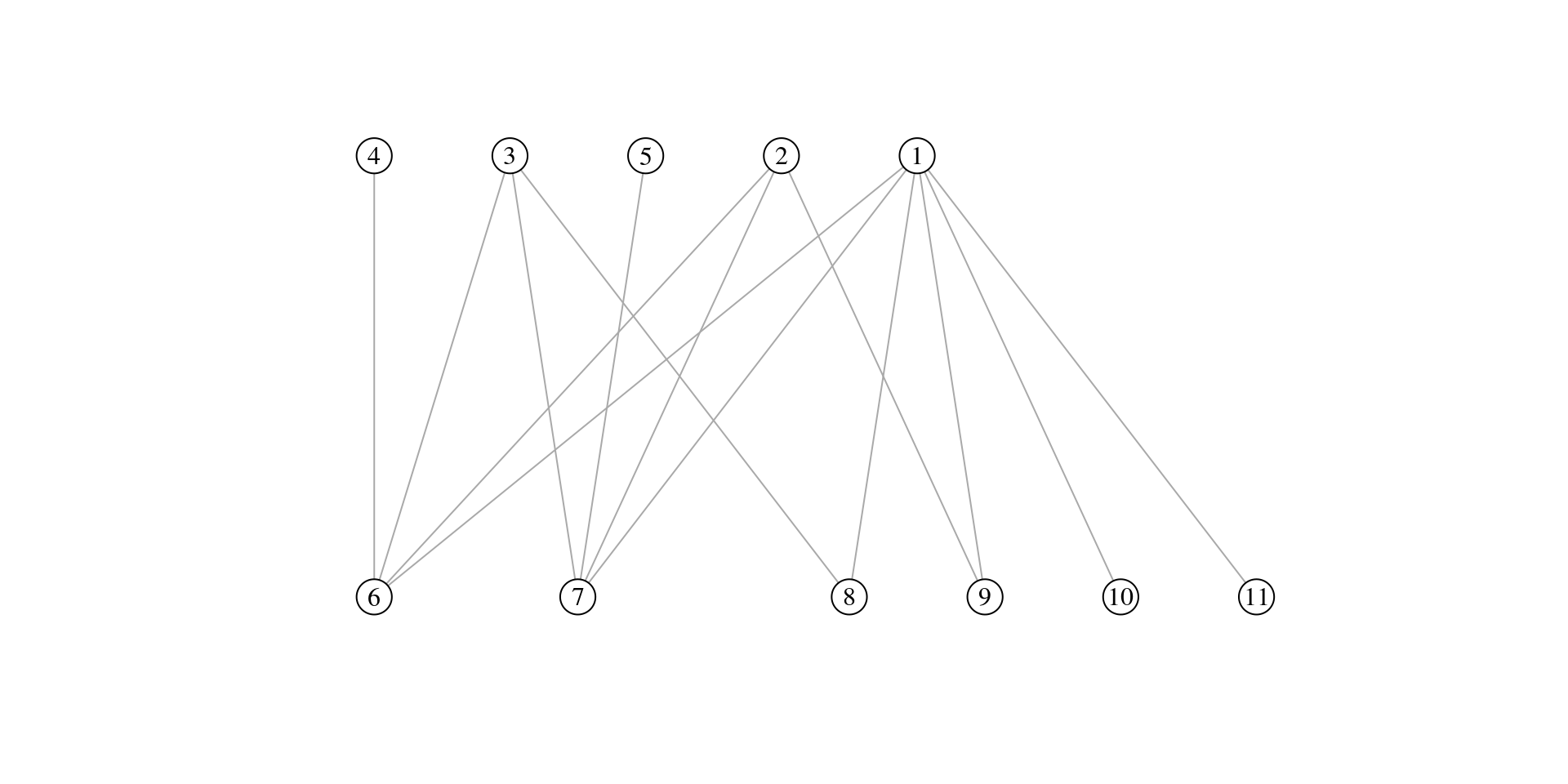
Please solve this exercise on a piece of paper. When you have finished, take a picture of your solution and upload it (along with the rest of your submission) into the corresponding folder on OLAT.
Exercise 2
Compute the nestedness of the bipartite graph defined by the incidence matrix \(B_2\).
\[ \\B_2 = \begin{bmatrix} 1 & 1 & 1 & 1 & 1 & 1 \\ 1 & 1 & 0 & 1 & 0 & 0 \\ 1 & 1 & 1 & 0 & 0 & 0 \\ 1 & 0 & 0 & 0 & 0 & 0 \\ 0 & 1 & 0 & 0 & 0 & 0 \\ \end{bmatrix} \]
Please solve this exercise on a piece of paper. When you have finished, take a picture of your solution and upload it (along with the rest of your submission) into the corresponding folder on OLAT.
4.3 Computing nestedness in R
We will now use R to quantify nestedness. Let’s start by loading some packages:
# Import the required libraries
library(rjson) # used for downloading networks from the Web of Life
library(igraph) # used for finding node partitions and plotting networks
library(dplyr) # used for wrangling data sets
Next we will download a seed dispersal network (M_SD_024) from the Web
of Life and use it to build a bipartite network. To do so, we will
follow the workflow outlined in the Toolkit for network analysis
chapter.
# Define the url associated with the network to be downloaded
json_url <- "https://www.web-of-life.es/get_networks.php?network_name=M_SD_024"

# Download the network (as a dataframe)
network_data <- jsonlite::fromJSON(json_url)

# Keep only the three relevant columns and use them to create the network
network <- network_data |>
  dplyr::select(species1, species2, connection_strength) |>
  # convert the connection_strength column to numeric
  dplyr::mutate(connection_strength = as.numeric(connection_strength)) |>
  graph_from_data_frame(directed = FALSE)

# Convert the network into bipartite format
V(network)$type <- bipartite.mapping(network)$type

# Assign different colours to plants and seed dispersers
V(network)$color <- ifelse(V(network)$type == TRUE, "blue", "orange")

# Plot network using bipartite layout
plot(network,
     layout=layout_as_bipartite,
     arrow.mode=0,
     vertex.label=NA,
     vertex.size=4,
     asp=0.2)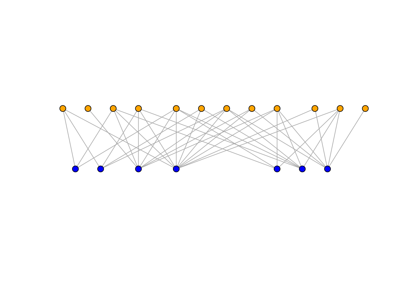
Now we will measure the nestedness of the network. To do so, we will use
the nestedness function found in the rweboflife package. Note that
the nestedness function measures the nestedness of an incidence
matrix. Thus, we will first have to convert our bipartite network into
an incidence matrix. Then we can measure how nested it is.
# Import the rweboflife package
library(rweboflife) # this package contains the nestdness function

# Convert the igraph bipartite network into an incidence matrix
network_matrix <- as_incidence_matrix(network, names=TRUE, sparse=FALSE)

# Compute network nestedness
network_nestedness <- rweboflife::nestedness(network_matrix)

# Print value
network_nestedness
## [1] 0.6318829We find that the network has a nestedness value of 0.63.
The nestedness function in rweboflife package uses the Fortuna et
al. (2019) nestedness measure. Below you can find the code of the
function that computes nestendess:
nestedness <- function(B){

  # Get number of rows and columns
  nrows <- nrow(B)
  ncols <- ncol(B)

  # Compute nestedness of rows
  nestedness_rows <- 0
  for(i in 1:(nrows-1)){
    for(j in (i+1): nrows){

      c_ij <- sum(B[i,] * B[j,])      # Number of interactions shared by i and j
      k_i <- sum(B[i,])               # Degree of node i
      k_j <- sum(B[j,])               # Degree of node j

      if (k_i == 0 || k_j==0) {next}  # Handle case if a node is disconnected

      o_ij <- c_ij / min(k_i, k_j)    # Overlap between i and j

      nestedness_rows <- nestedness_rows + o_ij
    }
  }

  # Compute nestedness of columns
  nestedness_cols <- 0
  for(i in 1: (ncols-1)){
    for(j in (i+1): ncols){

      c_ij <- sum(B[,i] * B[,j])      # Number of interactions shared by i and j
      k_i <- sum(B[,i])               # Degree of node i
      k_j <- sum(B[,j])               # Degree of node j
      if (k_i == 0 || k_j==0) {next}  # Handle case if a node is disconnected.

      o_ij <- c_ij / min(k_i, k_j)    # Overlap between i and j

      nestedness_cols <- nestedness_cols + o_ij
    }
  }

  # Compute nestedness of the network
  nestedness <- (nestedness_rows + nestedness_cols) /
    ((nrows * (nrows - 1) / 2) + (ncols * (ncols - 1) / 2))

  return(nestedness)
}4.4 Solutions
Exercise 1
For the bipartite graph drawn below:
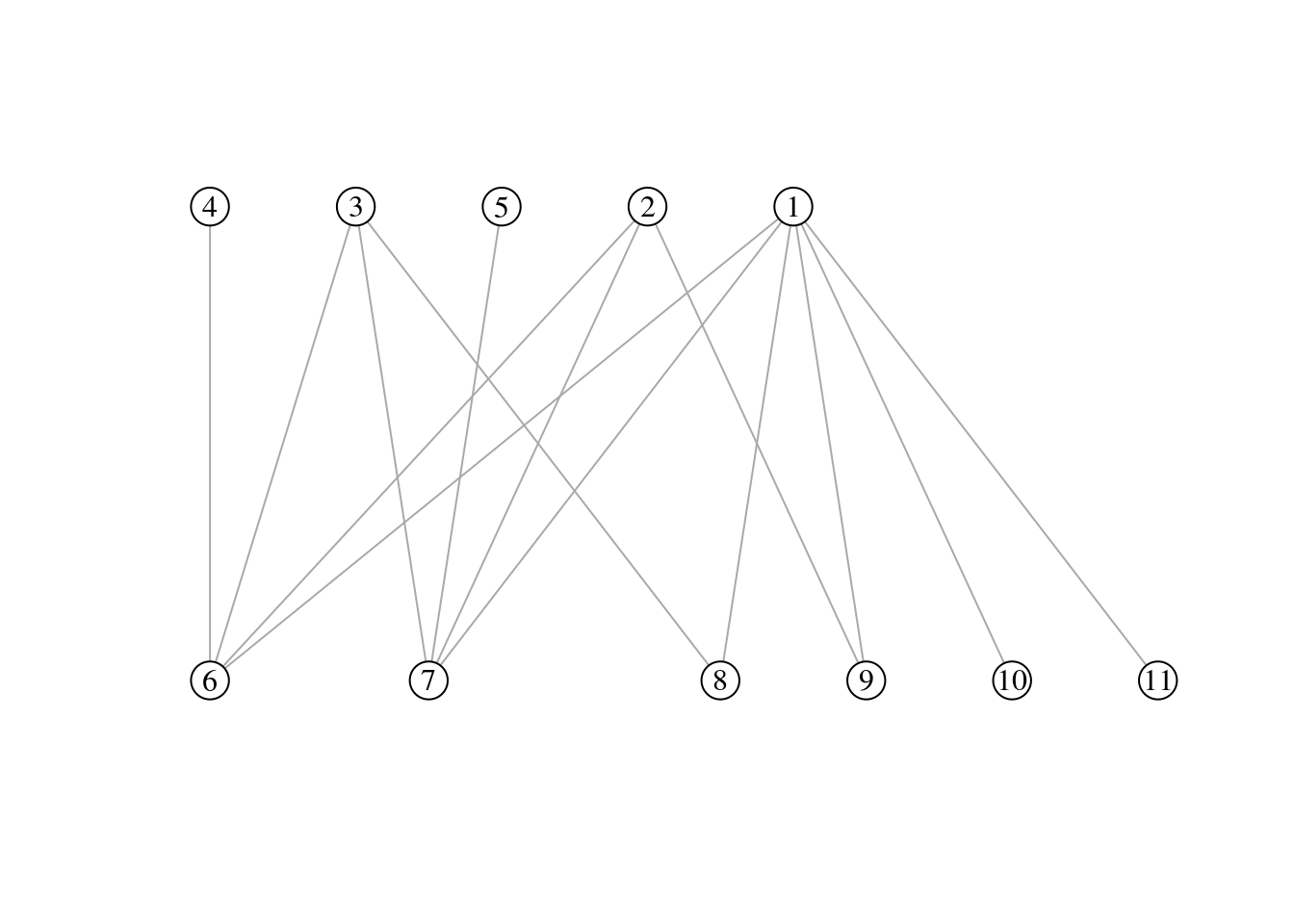
- write down the incidence matrix B
## 6 7 8 9 10 11
## 1 1 1 1 1 1 1
## 2 1 1 0 1 0 0
## 3 1 1 1 0 0 0
## 4 1 0 0 0 0 0
## 5 0 1 0 0 0 0- compute connectance C
## [1] "connectance: 0.47"Exercise 2
Compute the nestedness of the bipartite graph defined by the incidence matrix \(B_2\).
\[ \\B_2 = \begin{bmatrix} 1 & 1 & 1 & 1 & 1 & 1 \\ 1 & 1 & 0 & 1 & 0 & 0 \\ 1 & 1 & 1 & 0 & 0 & 0 \\ 1 & 0 & 0 & 0 & 0 & 0 \\ 0 & 1 & 0 & 0 & 0 & 0 \\ \end{bmatrix} \]
## [1] "nestedness: 0.92"Exercise 3
Use R to check the result you obtained in Exercise 2.
Hint: Use the following code to create the incidence matrix \(B_2\).
Then, calculate its nestedness using the nestedness function.
# Define the matrix
B_2 <- matrix(c(1,1,1,1,0,
                1,1,1,0,1,
                1,0,1,0,0,
                1,1,0,0,0,
                1,0,0,0,0,
                1,0,0,0,0),
              nrow=5, ncol=6)
# Compute its nestedness
B_2_nestedness <- rweboflife::nestedness(B_2)
# Print value
B_2_nestedness## [1] 0.9166667Exercise 4
For the mutualistic plant-pollinator network M_PL_052:
- Download the network from the Web of Life
# Define the url associated with the network to be downloaded
json_url <- "https://www.web-of-life.es/get_networks.php?network_name=M_PL_052"

# Download the network (as a dataframe)
M_PL_052_network_data <- jsonlite::fromJSON(json_url)

# Keep only the three relevant columns and use them to create the network
 M_PL_052_network <- M_PL_052_network_data |>
  dplyr::select(species1, species2, connection_strength) |>
  # convert the connection_strength column to numeric
  dplyr::mutate(connection_strength = as.numeric(connection_strength)) |>
  graph_from_data_frame(directed = FALSE)

# Convert the network into bipartite format
V(M_PL_052_network)$type <- bipartite.mapping(M_PL_052_network)$type- Compute connectance of the network.
# convert network to incidence matrix
M_PL_052_inc_matrix <- as_incidence_matrix(M_PL_052_network, sparse = FALSE)

# calculate connectance
M_PL_052_connectance_value <- sum(M_PL_052_inc_matrix)/
  (nrow(M_PL_052_inc_matrix) * ncol(M_PL_052_inc_matrix))

# print value
M_PL_052_connectance_value
## [1] 0.157265- Compute nestedness of the network.
# use the rweboflife package to compute nestedness
M_PL_052_nestedness_value <- rweboflife::nestedness(M_PL_052_inc_matrix)

# print value
M_PL_052_nestedness_value
## [1] 0.3509883