Chapter 9 Models of ecological dynamics
Subhendu Bhandary
session 28/03/2025
Introduction
In the realm of ecological network dynamics, the Lotka-Volterra model stands as a cornerstone, offering insights into the intricate interplay between species within ecological communities. This mathematical framework captures various dynamics that characterize ecosystems, ranging from stable equilibria to more complex phenomena such as limit cycles and chaos. At its core, the Lotka-Volterra model describes the population dynamics of interacting species, considering factors like predation, competition, and mutualism. Understanding the equilibrium points of this model sheds light on the stable coexistence of species, while exploring limit cycles reveals periodic fluctuations in population abundance. Moreover, the emergence of chaotic behavior underscores the inherent complexity of ecological systems, challenging traditional notions of predictability. Through the lens of stability analysis, researchers unravel the delicate balance between forces that promote species persistence and those that drive ecological change. In sum, the Lotka-Volterra model serves as a versatile tool for unraveling the dynamics of ecological networks, offering valuable insights into the resilience and fragility of natural ecosystems.
My tutorial section is split into mainly four sections:
Introduction to Population Dynamics: Discussing dynamics of single populations.
Multiple Species Dynamics: Exploring complex dynamics arising from interactions among multiple species.
Mutualistic Models: Examining mutualistic models and their implications for plant-pollinator species dynamics.
Role of Different Network Structures: Investigating how different levels of mutualistic strength influence species extinction across various ecological network structures.
Before we start, we load the packages we will be using for this exercise session:
9.1 Single population dynamics
The simplest case to study is that of a single population, in which scenario the equation transforms into the logistic growth equation: \[ \dfrac{dN}{dt} = N(t)(r+aN(t))\] Analytical solution: \[N(t)=\dfrac{r}{e^{-r(k+t)}-a}\] where \(k\) is a constant. By setting \(N(0)=N_0\) (i.e., providing an initial condition), solving for the constant and substituting, we obtain: \[N(t)=\dfrac{rN_0 e^{rt}}{r-aN_0(e^{rt}-1)}\] Thus, given the parameters \(r\) and \(a\), along with an initial condition, we can calculate the population size for any time \(t\). For instance, in R:
# define the differential equation
logistic_growth <- function(t, N, parameters){
  with(as.list(c(N, parameters)), {
    dNdt <- N * (r + a * N)
    list(dNdt)
  })
}
# define parameters, integration time, initial conditions
times <- seq(0, 50, by = 1)
N0 <- 0.05
r <- 0.3
a <- -0.1
parameters <- list(r = r, a = a)
# solve numerically
out <- deSolve::ode(y = N0, times = times,
           func = logistic_growth, parms = parameters,
           method = "ode45")
# now compute analytically
solution <- r * N0 * exp(r * times) / (r - a * N0 * (exp(r * times) - 1))
# use ggplot to plot
res <- dplyr::tibble(time = out[,1], N_t = out[,2], N_sol = solution)
ggplot(data = res) + aes(x = time, y = N_t) +
  geom_line() +
  geom_point(aes(x = time, y = N_sol), colour = "red", shape = 2) +
  ylab(expression("N(t)")) + xlab(expression("t"))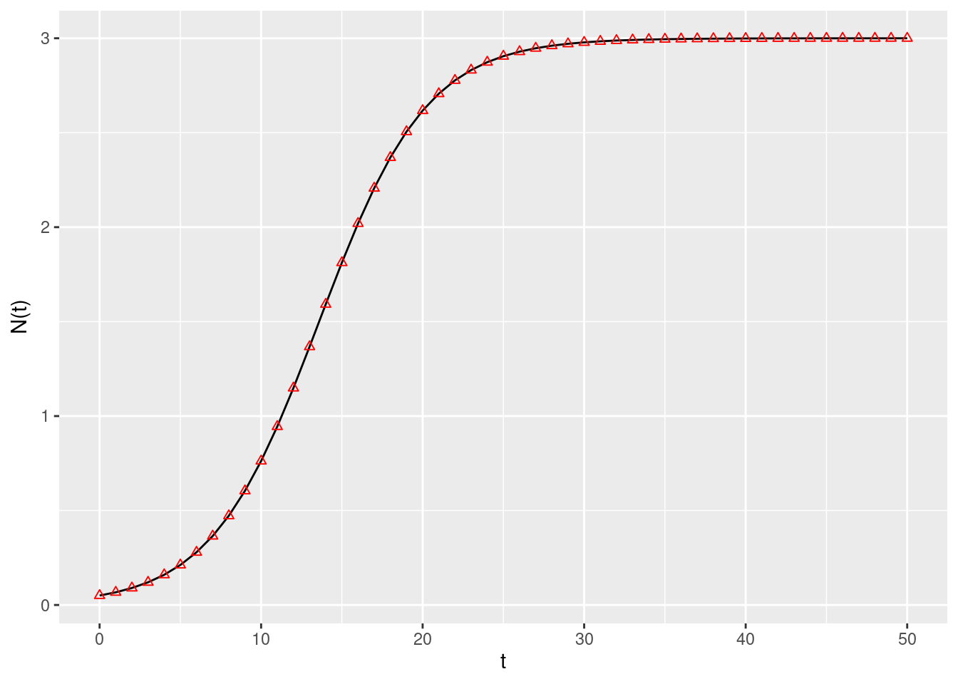
When \(a<0\) and \(r>0\), the population, beginning from any positive value, ultimately stabilizes at an equilibrium point. This equilibrium can be determined by setting the derivative of \(N(t)\) with respect to \(t\) equal to zero and considering \(N\neq 0\)
\[\dfrac{dN}{dt}=0\implies r+aN=0\] \[\implies N=-\dfrac{r}{a}\]
9.2 Multiple Species Dynamics
# Generalized Lotka-Volterra model
GLV <- function(t, N, parameters){
  with(as.list(c(N, parameters)), {
    N[N < 10^-8] <- 0 # prevent numerical problems
    dNdt <- N * (r + A %*% N)
    list(dNdt)
  })
}
# function to plot output
plot_ODE_output <- function(out){
  out <- as.data.frame(out)
  colnames(out) <- c("time", paste("sp", 1:(ncol(out) -1), sep = "_"))
  out <- as_tibble(out) |> gather(species, density, -time)
  pl <- ggplot(data = out) +
    aes(x = time, y = density, colour = species) +
    geom_line()
  show(pl)
  return(out)
}
# general function to integrate GLV
integrate_GLV <- function(r, A, N0, maxtime = 100, steptime = 0.5){
  times <- seq(0, maxtime, by = steptime)
  parameters <- list(r = r, A = A)
  # solve numerically
  out <- ode(y = N0, times = times,
           func = GLV, parms = parameters,
           method = "ode45")
  # plot and make into tidy form
  out <- plot_ODE_output(out)
  return(out)
}set.seed(1) # for reproducibility
r_1 <- rep(1, 3)
A_1 <- -matrix(c(10, 9, 5,
9, 10, 9,
5, 9, 10), 3, 3, byrow = TRUE)
# check the existence of feasible equilibrium
print(solve(A_1, -r_1)) # not feasible## [1] -0.08333333 0.25000000 -0.08333333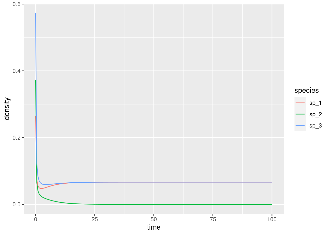
Stable Equilibrium
set.seed(2) # for reproducibility
r_2 <- rep(10, 3)
A_2 <- -matrix(c(10, 7, 12,
                 15, 10, 8,
                 7, 11, 10), 3, 3, byrow = TRUE)
# check the existence of feasible equilibrium
print(solve(A_2, -r_2)) # feasible
## [1] 0.1661130 0.3654485 0.4817276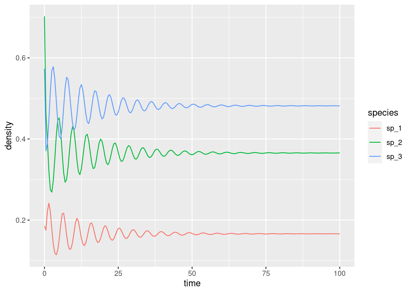
Stable Limit Cycles
set.seed(3) # for reproducibility
r_3 <- rep(1, 3)
A_3 <- -matrix(c(10, 6, 12,
                 14, 10, 2,
                 8, 18, 10), 3, 3, byrow = TRUE)
# check the existence of feasible equilibrium
print(solve(A_3, -r_3)) # feasible
## [1] 0.05714286 0.01428571 0.02857143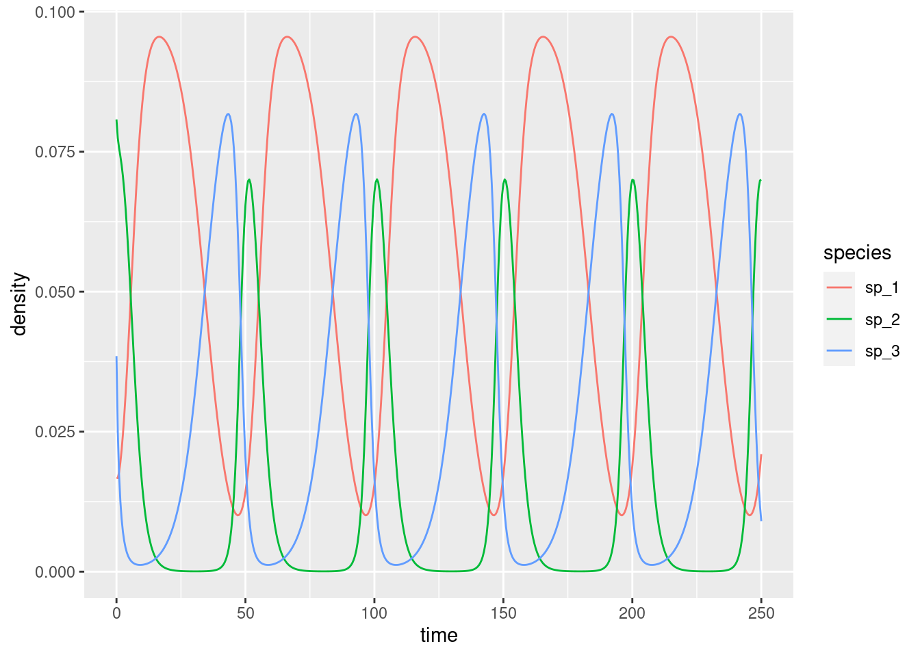
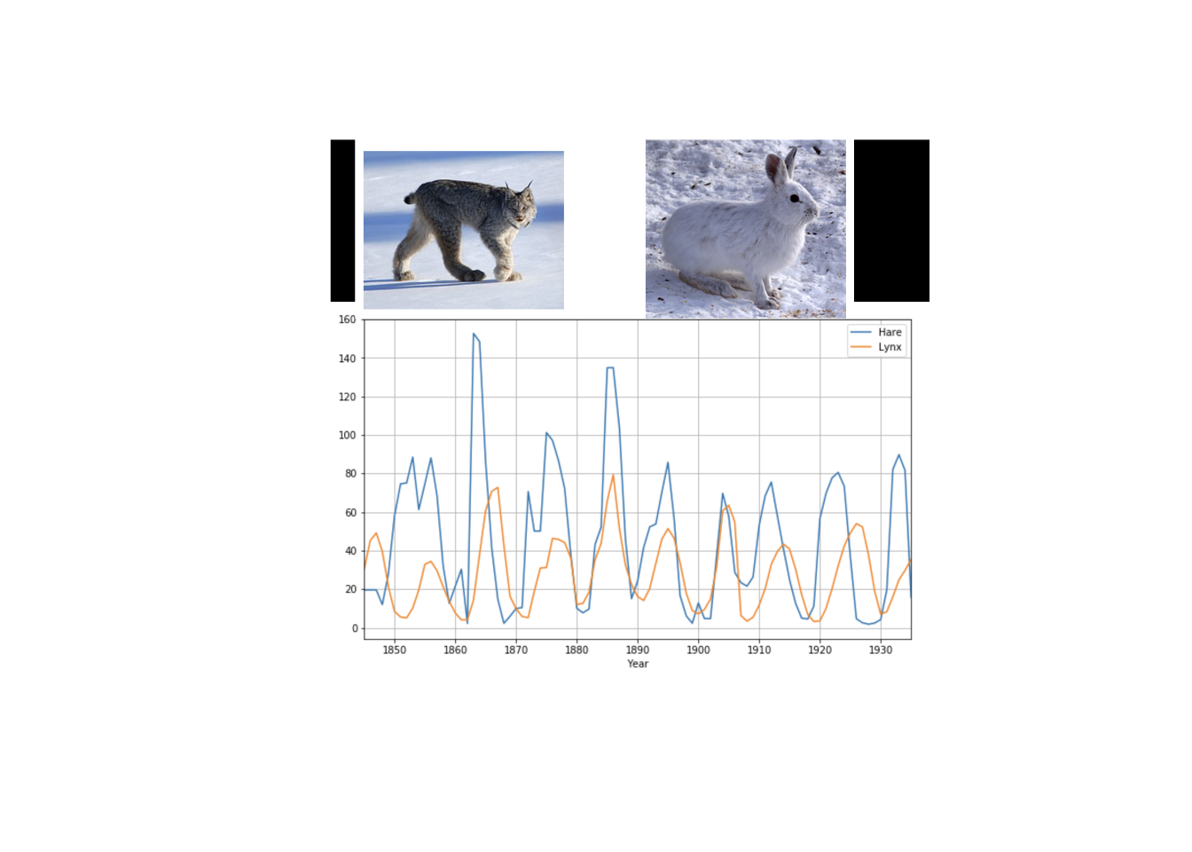
Note how the cycle dynamics obtained above compares with the time series representing Lynx-Hare population:
Chaos
set.seed(4) # for reproducibility
r_4 <- c(1, 0.72, 1.53, 1.27)
A_4 <- -matrix(c(1, 1.09, 1.52, 0,
                 0, 0.72, 0.3168, 0.9792,
                 3.5649, 0, 1.53, 0.7191,
                 1.5367, 0.6477, 0.4445, 1.27), 4, 4, byrow = TRUE)
# check the existence of feasible equilibrium
print(solve(A_4, -r_4)) # feasible
## [1] 0.3013030 0.4586546 0.1307655 0.3557416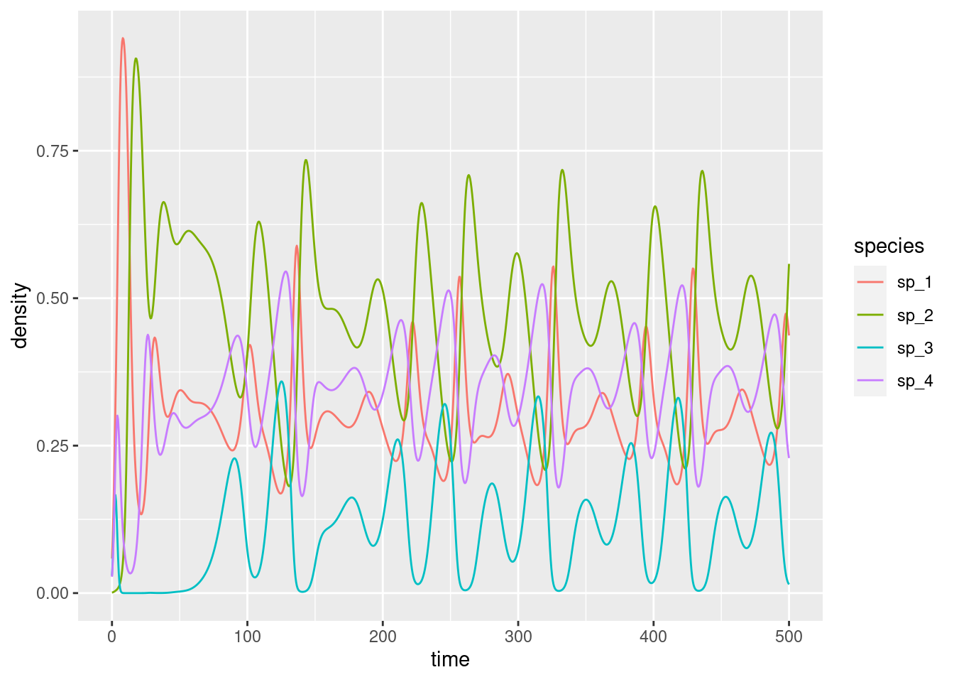
Predator-Prey Systems
library(deSolve)

LotVmod <- function (Time, State, Pars) {
  with(as.list(c(State, Pars)), {
    dN = N*(alpha - beta*P)
    dP = -P*(gamma - delta*N)
    return(list(c(dN, dP)))
  })
}

Pars <- c(alpha = 2, beta = .5, gamma = .2, delta = .6)
State <- c(N = 10, P = 10)
Time <- seq(0, 500, by = 1)

out <- as.data.frame(ode(func = LotVmod, y = State, parms = Pars, times = Time))

matplot(out[,-1], type = "l", xlab = "time", ylab = "population")
legend("topright", c("Cute bunnies", "Rabid foxes"), lty = c(1,2),
       col = c(1,2), box.lwd = 0)
9.3 Mutualistic Model
\[\dfrac{dN^{(A)}_{i}}{dt}=N^{(A)}_{i} \bigl(r^{(A)}_{i}-d^{(A)}_{i}-\sum_{j=1}^{S_A} \beta_{ij} N^{(A)}_{j} + \dfrac{\sum_{k=1}^{S_P} \gamma_{ik} N^{(P)}_{k}}{1+h \sum_{k=1}^{S_P} \gamma_{ik} N^{(P)}_{k}} \bigr) \] \[\dfrac{dN^{(P)}_{i}}{dt}=N^{(P)}_{i} \bigl(r^{(P)}_{i}-\sum_{j=1}^{S_P} \beta_{ij} N^{(P)}_{j} + \dfrac{\sum_{k=1}^{S_A} \gamma_{ik} N^{(A)}_{k}}{1+h \sum_{k=1}^{S_A} \gamma_{ik} N^{(A)}_{k}} \bigr) \] where \[\gamma_{ik}=\dfrac{\gamma_{0} a_{ik}}{k_{i}^\delta}\]
\(a_{ik}\) represents an element of the plant-pollinator network matrix \(A\). Here, \(a_{ik}=1\) if the \(i\)th species interacts with the \(k\)th species; otherwise, \(a_{ik}=0\). \(\gamma_{0}\) denotes the average mutualistic strength. We have already discussed the other parameters in our theoretical class.
Consider the following networks
- the pollination network B_2
- a perfectly nested network of the same dimensions as the network nested_B_2
- a randomized version of the network rnd_B_2
then solve the dynamics of plant, pollinator abundances.
# Define the bipartite matrix
B_2 <- matrix(c(1, 1, 1, 1, 0,
                1, 1, 1, 0, 1,
                1, 0, 1, 0, 0,
                1, 1, 0, 0, 0,
                1, 0, 0, 0, 0,
                1, 0, 0, 0, 0), nrow = 5, ncol = 6)

# Load the perfect_nested function from our toolbox
source("~/ecological_networks_2025/downloads/Functions/helper.R")
# Build a perfectly nested network, the function takes as arguments the number
# of rows and columns of the target matrix.
nested_B_2 <- perfect_nested(nrow(B_2), ncol(B_2))
set.seed(10)
rnd_B_2 <- rweboflife::null_model(B_2, model = "equifrequent")

library(rweboflife)
# Compute network nestedness
rweboflife::nestedness(nested_B_2)
## [1] 1## [1] 0.4666667## [1] 0.9166667# Calculate dimensions
dim_mat <- dim(B_2)
SP <- dim_mat[1]
SA <- dim_mat[2]
S <- SA + SP
lv_bipartite2_heterogenity <- function(t, N, p) {
N_a <- N[1:p$SA]
N_p <- N[(p$SA + 1):(p$SA + p$SP)]
num <- p$gammaAP[1:p$SA, ] %*% N[(p$SA + 1):(p$SA + p$SP)]
num1 <- p$gammaPA[1:p$SP, ] %*% N[1:p$SA]
den <- 1 + p$h[1:p$SA] * num
den1 <- 1 + p$h[(p$SA + 1):(p$SA + p$SP)] * num1
numden <- num / den
numden1 <- num1 / den1
dN_a <- N_a *
(p$r[1:p$SA] - p$r_d[1:p$SA] - p$betaA[1:p$SA, ] %*% N[1:p$SA] + numden)
dN_p <- N_p *
(p$r[(p$SA + 1):(p$SA + p$SP)] - p$betaP[1:p$SP, ] %*% N[(p$SA + 1):(p$SA + p$SP)] +
numden1)
dN <- c(dN_a, dN_p)
return(list(dN))
}
calculate_parameters <- function(B, gamma_0) {
dim_mat <- dim(B)
SP <- dim_mat[1]
SA <- dim_mat[2]
S <- SA + SP
k1 <- rowSums(B)
k2 <- colSums(B)
t <- 0.5
gammaPA <- gamma_0 * (B / (k2^t))
gammaAP <- gamma_0 * (t(B) / (k1^t))
betaA <- matrix(0.0, nrow = SA, ncol = SA)
diag(betaA) <- 1
betaP <- matrix(0.0, nrow = SP, ncol = SP)
diag(betaP) <- 1
r <- c(rep(-0.3, S))
r_d <- c(rep(0.0, SA)) # Fixed r_d as 0
h <- c(rep(0.2, S))
return(list(SA = SA, SP = SP, S = S, r = r, r_d = r_d, betaA = betaA,
betaP = betaP, h = h, gammaAP = gammaAP, gammaPA = gammaPA))
}
# Define time parameters
tbegin <- 0.0
tend <- 100
tstep <- 0.1
trange <- seq(tbegin, tend, by = tstep)
# Initial conditions
mu_N0 <- 4
N0 <- mu_N0 * runif(S)Solve the mutualistic model for mutualistic strength \(\gamma_0=1\)
parameters <- calculate_parameters(B_2, 1)
    out <- ode(
      y = mu_N0 * runif(parameters$S),
      times = trange,
      func = lv_bipartite2_heterogenity,
      parms = parameters
    )
Plot plant pollinator abundances with time
# Set up the layout for the subplot with two columns
par(mfrow = c(1, 2))

# Plot for pollinators
plot(out[,1], out[, 2], type = "n", xlab = "time",
     ylab = "Abundance", main = "Pollinator Abundances", ylim = c(0, 5))
for (i in 2:(SA + 1)) {
  lines(out[,1], out[, i], type = "l", lwd = 2, col = rainbow(SA - 1)[i - 1])
}
legend("topright", legend = paste("Pollinator", 1:(SA)),
       col = rainbow(SA), lty = 1)

# Plot for plants
plot(out[,1], out[, (SA + 2)], type = "n", xlab =  "time",
     ylab = "Abundance", main = "Plant Abundances", ylim = c(0, 5))
for (i in (SA + 2):ncol(out)) {
  lines(out[,1], out[, i], type = "l", lwd = 2,
        col = rainbow(ncol(out) - SA - 1)[i - SA - 1])
}
legend("topright", legend = paste("Plant", 1:(ncol(out) - SA - 1)),
       col = rainbow(ncol(out) - SA - 1), lty = 1)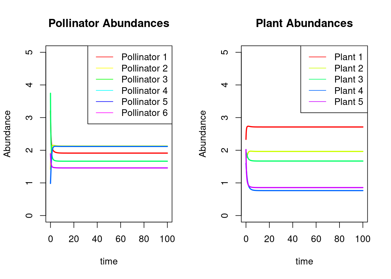
9.4 Role of network structure on Collapse
Plot plant and pollinator abundance while varying \(\gamma_0\), taking species abundance for each \(\gamma_0\) ranging from \(3\) to \(0\). Investigate the collapse phenomenon across three distinct network structures: B_2, nested_B_2, and rnd_B_2.
# Load required libraries
library(deSolve)
library(tibble)
library(ggplot2)


# Define the bipartite matrix
B_2 <- matrix(c(1, 1, 1, 1, 0,
                1, 1, 1, 0, 1,
                1, 0, 1, 0, 0,
                1, 1, 0, 0, 0,
                1, 0, 0, 0, 0,
                1, 0, 0, 0, 0), nrow = 5, ncol = 6)

# Calculate parameters
#parameters <- calculate_parameters(B_2)

# Define the ODE function
lv_bipartite2_heterogenity <- function(t, N, p) {
  N_a <- N[1:p$SA]
  N_p <- N[(p$SA + 1):(p$SA + p$SP)]

  num <- p$gammaAP[1:p$SA, ] %*% N[(p$SA + 1):(p$SA + p$SP)]
  num1 <- p$gammaPA[1:p$SP, ] %*% N[1:p$SA]
  den <- 1 + p$h[1:p$SA] * num
  den1 <- 1 + p$h[(p$SA + 1):(p$SA + p$SP)] * num1

  numden <- num / den
  numden1 <- num1 / den1

  dN_a <- N_a *
    (p$r[1:p$SA] - p$r_d[1:p$SA] - p$betaA[1:p$SA, ] %*% N[1:p$SA] + numden)
  dN_p <- N_p *
    (p$r[(p$SA + 1):(p$SA + p$SP)] - p$betaP[1:p$SP, ] %*% N[(p$SA + 1):(p$SA + p$SP)] +
       numden1)

  dN <- c(dN_a, dN_p)
  return(list(dN))
}

calculate_parameters <- function(B, gamma_0) {
  dim_mat <- dim(B)
  SP <- dim_mat[1]
  SA <- dim_mat[2]
  S <- SA + SP

  k1 <- rowSums(B)
  k2 <- colSums(B)

  t <- 0.5
  gammaPA <- gamma_0 * (B / (k2^t))
  gammaAP <- gamma_0 * (t(B) / (k1^t))

  betaA <- matrix(0.0, nrow = SA, ncol = SA)
  diag(betaA) <- 1
  betaP <- matrix(0.0, nrow = SP, ncol = SP)
  diag(betaP) <- 1

  r <- c(rep(-0.3, S))
  r_d <- c(rep(0.0, SA)) # Fixed r_d as 0
  h <- c(rep(0.2, S))

  return(list(SA = SA, SP = SP, S = S, r = r, r_d = r_d, betaA = betaA,
              betaP = betaP, h = h, gammaAP = gammaAP, gammaPA = gammaPA))
}

# Solving ODE for varying gamma_0 values
# Define gamma_0 values
gamma_0_values <- seq(3, 0, by = -0.1)
end_values <- NULL

# Function to solve ODE and store end values of plant and pollinator abundances
solve_ODE_store_end_values <- function(B, gamma_0_values, trange) {
  end_values <- data.frame(gamma_0 = numeric(),
                           Pollinator = numeric(), Plant = numeric())
  for (gamma_0 in gamma_0_values) {
    parameters <- calculate_parameters(B, gamma_0)
    out <- ode(
      y = mu_N0 * runif(parameters$S),
      times = trange,
      func = lv_bipartite2_heterogenity,
      parms = parameters
    )
    plant_end_values <- tail(out[, (parameters$SA + 2):(parameters$SA +
                                                          parameters$SP + 1)], 1)
    pollinator_end_values <- tail(out[, 2:(parameters$SA + 1)], 1)
    end_values <- rbind(end_values, c(gamma_0, pollinator_end_values,
                                      plant_end_values))
  }
  colnames(end_values) <- c("gamma_0", paste("Pollinator", 1:parameters$SA),
                            paste("Plant", 1:parameters$SP))
  return(end_values)
}


# Solve ODE and store end values
end_values <- solve_ODE_store_end_values(B_2, gamma_0_values, trange)
#print(end_values)
nested_end_values <- solve_ODE_store_end_values(nested_B_2, gamma_0_values, trange)

rnd_end_values <- solve_ODE_store_end_values(rnd_B_2, gamma_0_values, trange)
dim_mat <- dim(B_2)
SP <- dim_mat[1]
SA <- dim_mat[2]
# Define colors for pollinators and plants
pollinator_color <- "blue"
plant_color <- "green"
# Create an empty plot canvas
plot(end_values$gamma_0, end_values[, 2], type = "n",
xlab = expression(paste(gamma[0])), ylab = "Abundance",
main = "B_2 :Plant and Pollinator Abundances ", ylim = c(0, 5))
# Plot end values of pollinators
for (i in 3:(SA + 1)) {
lines(end_values$gamma_0, end_values[, i],
type = "l", lwd = 2, col = pollinator_color)
}
# Plot end values of plants
for (i in (SA + 2):ncol(end_values)) {
lines(end_values$gamma_0, end_values[, i],
type = "l", lwd = 2, col = plant_color)
}
# Add legend
legend("topright", legend = c("Pollinator", "Plant"),
col = c(pollinator_color, plant_color), lty = 1)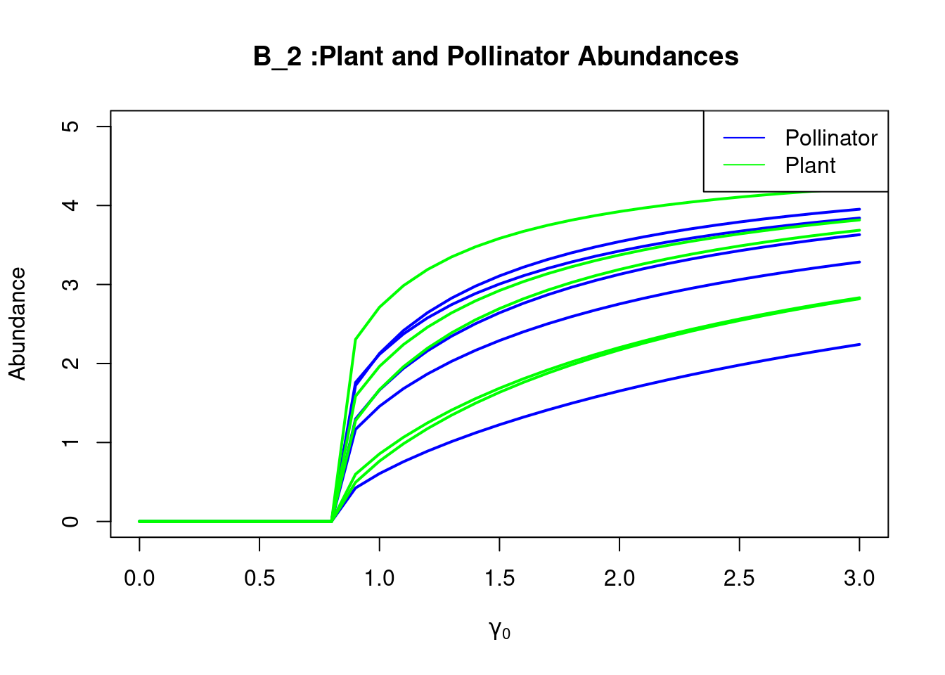
  dim_mat <- dim(nested_B_2)
  SP <- dim_mat[1]
  SA <- dim_mat[2]
# Define colors for pollinators and plants
pollinator_color <- "blue"
plant_color <- "green"

# Create an empty plot canvas
plot(nested_end_values$gamma_0, nested_end_values[, 2], type = "n",
     xlab =  expression(paste(gamma[0])), ylab = "Abundance",
     main = " nested_B_2 :Plant and Pollinator Abundances", ylim = c(0, 5))

# Plot end values of pollinators
for (i in 3:(SA + 1)) {
  lines(nested_end_values$gamma_0, nested_end_values[, i],
        type = "l", lwd = 2, col = pollinator_color)
}

# Plot end values of plants
for (i in (SA + 2):ncol(end_values)) {
  lines(nested_end_values$gamma_0, nested_end_values[, i],
        type = "l", lwd = 2, col = plant_color)
}

# Add legend
legend("topright", legend = c("Pollinator", "Plant"),
       col = c(pollinator_color, plant_color), lty = 1)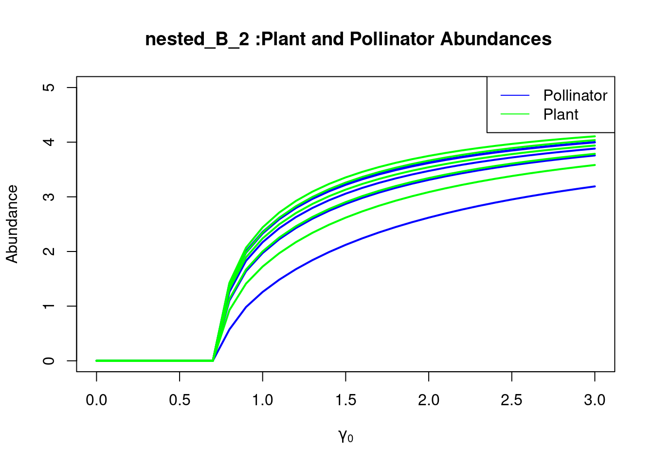
  dim_mat <- dim(rnd_B_2)
  SP <- dim_mat[1]
  SA <- dim_mat[2]
# Define colors for pollinators and plants
pollinator_color <- "blue"
plant_color <- "green"

# Create an empty plot canvas
plot(rnd_end_values$gamma_0, rnd_end_values[, 2], type = "n",
     xlab =  expression(paste(gamma[0])), ylab = "Abundance",
     main = " rnd_B_2 :Plant and Pollinator Abundances", ylim = c(0, 5))

# Plot end values of pollinators
for (i in 3:(SA + 1)) {
  lines(rnd_end_values$gamma_0, rnd_end_values[, i], type = "l",
        lwd = 2, col = pollinator_color)
}

# Plot end values of plants
for (i in (SA + 2):ncol(end_values)) {
  lines(rnd_end_values$gamma_0, rnd_end_values[, i], type = "l",
        lwd = 2, col = plant_color)
}

# Add legend
legend("topright", legend = c("Pollinator", "Plant"),
       col = c(pollinator_color, plant_color), lty = 1)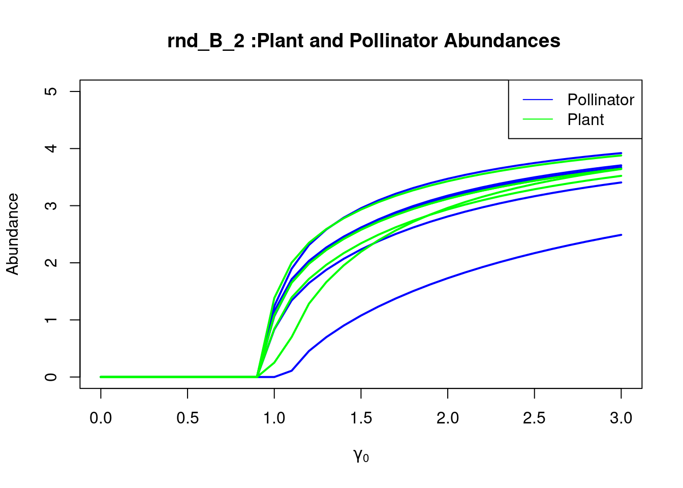
Exercises
Nestedness of an Emperical Network and its perfectly nested couterpart
Load the Empirical Pollination Network and Calculate Nestedness Value:
\(\bullet\) Begin by downloading the empirical pollination network data, denoted
as M_PL_006, into your R script and convert this matrix into an incidence
matrix representation (see session Toolkit for network analysis).
\(\bullet\) Calculate the nestedness value of the network matrix using appropriate algorithms or packages.
\(\bullet\) Generate one perfectly nested matrix with the same dimensions as
the M_PL_006 matrix and check that its nestedness value is actually one.
# Import the packages needed for this part
library(rjson)
library(dplyr)
library(rweboflife)
library(bipartite)
library(ggplot2)
library(latex2exp)
# define the base url
base_url <- "https://www.web-of-life.es/"
# Define the url associated with the network to be downloaded
json_url <- "https://www.web-of-life.es/get_networks.php?network_name=M_PL_006"
# Download the network (as a dataframe)
M_PL_006_nw <- jsonlite::fromJSON(json_url)
class(M_PL_006_nw$connection_strength) <-"numeric"

# Select the relevant columns and create the igraph object
M_PL_006_graph <- M_PL_006_nw |>
  dplyr::select(species1, species2, connection_strength) |>
  graph_from_data_frame(directed=FALSE)

# get info about species
my_info <- read.csv(paste0(base_url,"get_species_info.php?network_name=M_PL_006"))

for(id in seq(1,dim(my_info)[1])){
  v_type <- !(my_info$is.resource[id] |> as.logical()) # 0/1 converted to FALSE/TRUE
  v_name <- my_info$species[id]
  # Add the "type" attribute to the vertices of the graph
  V(M_PL_006_graph)[name==v_name]$type <- v_type
}


is_bipartite(M_PL_006_graph)
## [1] TRUE# convert the igraph object into incidence matrix
inc_matrix <- as_incidence_matrix(
M_PL_006_graph,
attr = "connection_strength",
names = TRUE,
sparse = FALSE
)
# convert elements into numeric values
class(inc_matrix) <-"numeric"
# remove NA values (previous empty strings)
inc_matrix[which(is.na(inc_matrix) == T)]<-0
# check dimensions and compare with the number of species on the Web interface
#dim(inc_matrix)
# Binarize the matrix
B_inc_matrix <- as.matrix((inc_matrix>0))
class(B_inc_matrix) <- "numeric"
rownames(B_inc_matrix) <- NULL
colnames(B_inc_matrix) <- NULL
#print(B_inc_matrix)
# build PERFECT nested loading a function from the helper.R file
source("~/ecological_networks_2024/downloads/Functions/helper.R")
nested_inc_mat <- perfect_nested(nrow(B_inc_matrix), ncol(B_inc_matrix))
#print(nested_inc_mat)Hint: Use the function rweboflife::nestedness to compute the nestedness of the 2 different matrices.
## [1] 1## [1] 0.6541883Collapse in Emperical Network
Simulate Dynamics and Plot Time Series for Different Mutualistic Strengths:
\(\bullet\) Using the M_PL_006 matrix, simulate the dynamics of the system over
time for both low (\(\gamma_0 = 0.3\)) and high (\(\gamma_0 = 2\)) mutualistic strengths.
\(\bullet\) Plot the time series for the species abundances in each scenario.
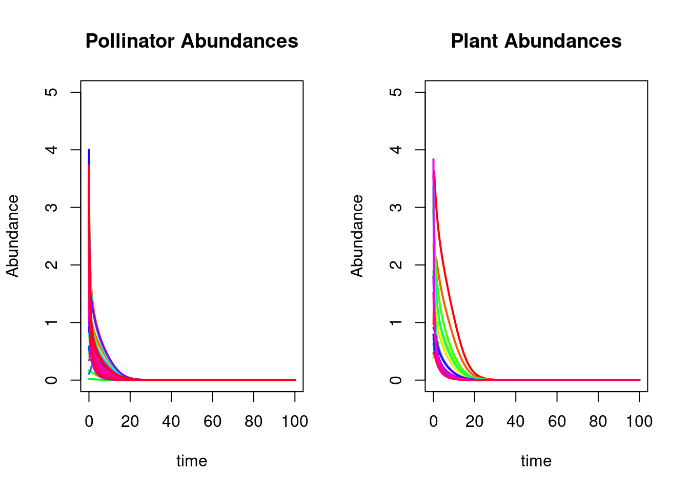
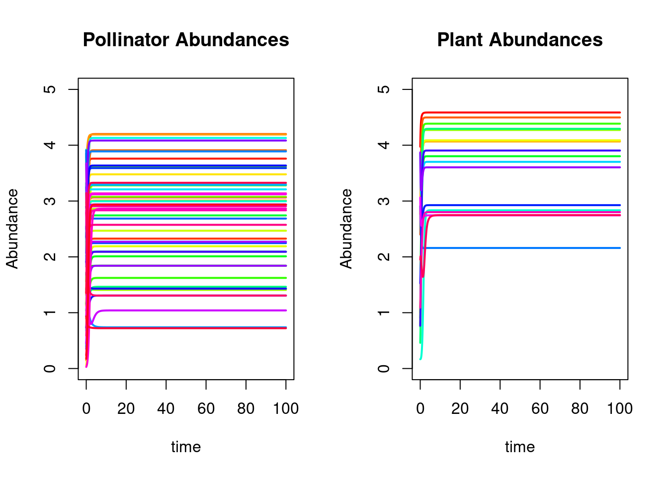
\(\bullet\) After having obtained the plant-pollinator abundances over time, discuss the type of dynamics they exhibit: stable equilibrium, limit cycle, or chaotic behavior?
ANSWER: Stable equilibrium
SOLUTION FOR \(\gamma_{0}=0.3\)
 parameters <- calculate_parameters(B_inc_matrix, 0.3)
    out <- ode(
      y = mu_N0 * runif(parameters$S),
      times = trange,
      func = lv_bipartite2_heterogenity,
      parms = parameters
    )

    # Set up the layout for the subplot with two columns
par(mfrow = c(1, 2))
SA<-parameters$SA
SP<-parameters$SP
S<-parameters$S
# Plot for pollinators
plot(out[,1], out[, 2], type = "n", xlab = "time",
     ylab = "Abundance", main = "Pollinator Abundances", ylim = c(0, 5))
for (i in 2:(SA + 1)) {
  lines(out[,1], out[, i], type = "l", lwd = 2, col = rainbow(SA - 1)[i - 1])
}


# Plot for plants
plot(out[,1], out[, (SA + 2)], type = "n", xlab =  "time",
     ylab = "Abundance", main = "Plant Abundances", ylim = c(0, 5))
for (i in (SA + 2):ncol(out)) {
  lines(out[,1], out[, i], type = "l", lwd = 2,
        col = rainbow(ncol(out) - SA - 1)[i - SA - 1])
}
SOLUTION FOR \(\gamma_{0}=2\)
 parameters <- calculate_parameters(B_inc_matrix, 2)
    out <- ode(
      y = mu_N0 * runif(parameters$S),
      times = trange,
      func = lv_bipartite2_heterogenity,
      parms = parameters
    )

    # Set up the layout for the subplot with two columns
par(mfrow = c(1, 2))
SA<-parameters$SA
SP<-parameters$SP
S<-parameters$S
# Plot for pollinators
plot(out[,1], out[, 2], type = "n", xlab = "time",
     ylab = "Abundance", main = "Pollinator Abundances", ylim = c(0, 5))
for (i in 2:(SA + 1)) {
  lines(out[,1], out[, i], type = "l", lwd = 2, col = rainbow(SA - 1)[i - 1])
}
#legend("topright", legend = paste("Pollinator", 1:(SA)),
#col = rainbow(SA), lty = 1)

# Plot for plants
plot(out[,1], out[, (SA + 2)], type = "n", xlab =  "time",
     ylab = "Abundance", main = "Plant Abundances", ylim = c(0, 5))
for (i in (SA + 2):ncol(out)) {
  lines(out[,1], out[, i], type = "l", lwd = 2,
        col = rainbow(ncol(out) - SA - 1)[i - SA - 1])
}
#legend("topright", legend = paste("Plant", 1:(ncol(out) - SA - 1)),
#col = rainbow(ncol(out) - SA - 1), lty = 1)
# Solve ODE and store end values
end_values <- solve_ODE_store_end_values(B_inc_matrix, gamma_0_values, trange)
nested_end_values <- solve_ODE_store_end_values(nested_inc_mat, gamma_0_values, trange) Analyzing Abundance Patterns:
\(\bullet\) Compare the abundance patterns of the species between the low and high mutualistic strength scenarios.
\(\bullet\) Comment on any significant differences or similarities observed in species dynamics, considering factors such as diversity, stability, and overall ecosystem dynamics.
Varying \(\gamma_0\) and plotting Abundance for M_PL_006:
\(\bullet\) Plot the abundance dynamics for various values of \(\gamma_0\), ranging from high to low(\(3\) to \(0\)), to observe how changes in mutualistic strength influence species interactions and ecosystem dynamics.
M_PL_006_Collapse:
  dim_mat <- dim(B_inc_matrix)
  SP <- dim_mat[1]
  SA <- dim_mat[2]
# Define colors for pollinators and plants
pollinator_color <- "blue"
plant_color <- "green"

# Create an empty plot canvas
plot(end_values$gamma_0, end_values[, 2], type = "n",
     xlab =  expression(paste(gamma[0])), ylab = "Abundance",
     main = " Plant and Pollinator Abundances", ylim = c(0, 5))

# Plot end values of pollinators
for (i in 3:(SA + 1)) {
  lines(end_values$gamma_0, end_values[, i],
        type = "l", lwd = 2, col = pollinator_color)
}

# Plot end values of plants
for (i in (SA + 2):ncol(end_values)) {
  lines(end_values$gamma_0, end_values[, i],
        type = "l", lwd = 2, col = plant_color)
}

# Add legend
legend("topright", legend = c("Pollinator", "Plant"),
       col = c(pollinator_color, plant_color), lty = 1)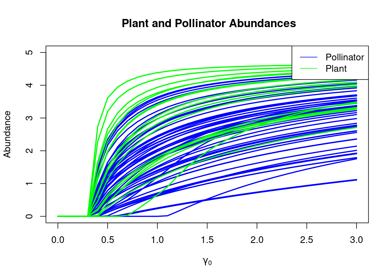
Analyzing Nestedness and Collapse Point:
\(\bullet\) Identify and discuss the collapse point of MPL_006 and the nested matrix. The collapse point refers to the threshold mutualistic strength \(\gamma_0\) at which the network transitions from an upper stable to extinction state for all species.
\(\bullet\) Evaluate the implications of the collapse point on stability, ecosystem resilience, providing insights into the underlying mechanisms driving ecosystem dynamics in pollination networks.
  dim_mat <- dim(nested_inc_mat)
  SP <- dim_mat[1]
  SA <- dim_mat[2]
# Define colors for pollinators and plants
pollinator_color <- "blue"
plant_color <- "green"

# Create an empty plot canvas
plot(nested_end_values$gamma_0, nested_end_values[, 2],
     type = "n", xlab =  expression(paste(gamma[0])),
     ylab = "Abundance", main = "Plant and Pollinator Abundances", ylim = c(0, 5))

# Plot end values of pollinators
for (i in 3:(SA + 1)) {
  lines(nested_end_values$gamma_0, nested_end_values[, i],
        type = "l", lwd = 2, col = pollinator_color)
}

# Plot end values of plants
for (i in (SA + 2):ncol(nested_end_values)) {
  lines(nested_end_values$gamma_0, nested_end_values[, i],
        type = "l", lwd = 2, col = plant_color)
}

# Add legend
legend("topright", legend = c("Pollinator", "Plant"),
       col = c(pollinator_color, plant_color), lty = 1)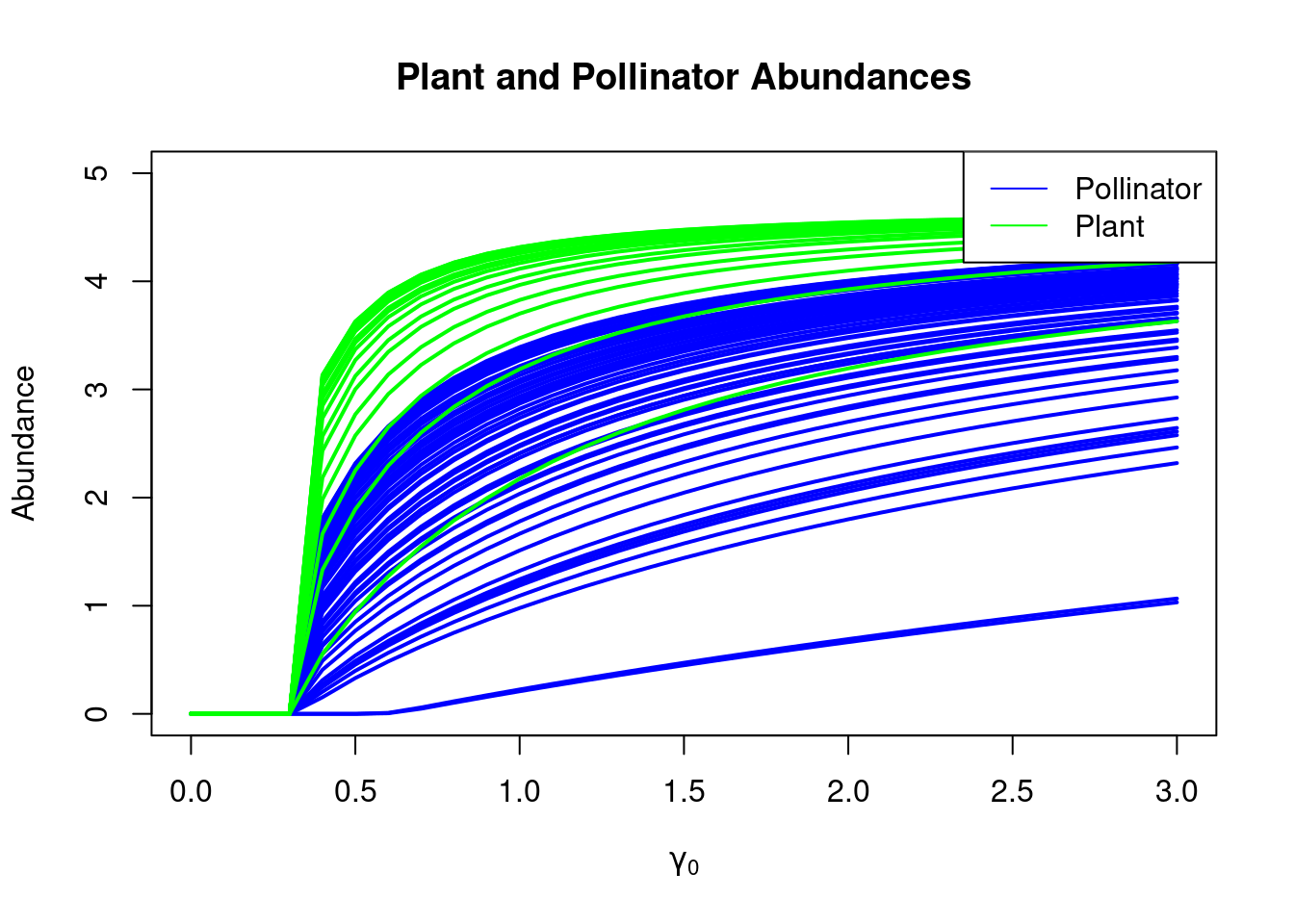
Solutions
The expected output of the plots is displayed in the section Exercises along with the code chunk to produce it.
In the following we will reply to the questions that were posed, point by point.
Collapse in Emperical Network
Analyzing Abundance Patterns:
\(\bullet\) Compare the abundance patterns of the species between the low and high mutualistic strength scenarios.
ANSWER: The plant and pollinator abundances at high mutualistic strength will be more than at low mutualistic strength.
\(\bullet\) Comment on any significant differences or similarities observed in species dynamics, considering factors such as diversity, stability, and overall ecosystem dynamics.
ANSWER: For high mutualistic strength there is more diversity in species abundance than in low mutualistic strength.
Analyzing Nestedness and Collapse Point:
\(\bullet\) Identify and discuss the collapse point of MPL_006 and the nested matrix. The collapse point refers to the threshold mutualistic strength \(\gamma_0\) at which the network transitions from an upper stable to extinction state for all species.
ANSWER: The collapse occurs at lower value of \(\gamma_0\) for the perfectly nested matrix than in MPL_006 network. Most species experiences collapse at the same value of \(\gamma_0\) for the perfectly nested matrix, while there is a spreading in the case of the empirical network MPL_006.
\(\bullet\) Evaluate the implications of the collapse point on stability, ecosystem resilience, providing insights into the underlying mechanisms driving ecosystem dynamics in pollination networks.
ANSWER: The results obtained above show that the resilienace of ecological networks increases with increasing nestedness.