Chapter 6 Comparing networks in space
Subhendu Bhandary
session 21/03/2025
Slides for this exercise session are available here.
6.1 Introduction
In ecology, we explore how similar two communities are through the concept of beta diversity (β-diversity). β-diversity is the species turnover between two different communities. This metric refers to how similar or how stable the communities are through space or time. Traditionally, community ecologists have analysed spatial and temporal differences only in species composition, without considering the changes in species interactions or species roles within assemblages (Poisot et al., 2012).
Quantifying to what extent interaction realization varies, both between sites (or across time), and when compared to the metaweb, can help us understand environmental and human impacts on network structure.
The recent applications for quantifying interaction β-diversity support the growing realization that links in a network are not merely contingent on two species co-occurring but are influenced by a series of other factors, which vary over space and time, and that can promote a rearrangement (rewiring) of the interactions (Poisot et al., 2012).
Through the following exercise session, we will learn how to analyse and interpret the interaction β-diversity and how to relate it to the distribution of communities in space.
- Poisot T., Canard D.M., Mouquet, N., Gravel D.: The dissimilarity of species interaction networks. Ecology Letters, 1353-1361 (2012). DOI 10.1111/ele.12002
6.2 Interaction β-diversity
Poisot et al. (2012) proposed that differences in interactions between networks originate from differences in species composition, and because the same species may interact differently in two different communities. Therefore, the interaction β-diversity can be partitioned as:
\[β_{WN} = β_{ST} + β_{OS}\]
Where \(β_{WN}\) is the total dissimilarity of interactions between networks that results from:
\(β_{ST}\): the dissimilarity of interactions due to differences in species composition (species turnover), and
\(β_{OS}\), the dissimilarity of interactions due to rearrangement of interactions (rewiring).
To calculate \(β_{WN}\) and \(β_{OS}\), we will adopt the Whittaker’s dissimilarity measure \(β_{W}\):
\[β_{W}=\frac{a+b+c}{(2a+b+c)/2} - 1\]
Where: \(a\) is the number of interactions that are shared between two networks, \(b\) is the number of interactions that are unique to network 1, and \(c\) is the number of interactions that are unique to network 2.
Note that, while other dissimilarity measures exist, Whittaker’s is widely used in ecology.
Because differences in network structure can arise either through changes in species compositions or realized interactions, there is no obvious analytical solution for \(β_{ST}\). It is calculated as the difference between \(β_{WN}\) and \(β_{OS}\).
6.3 β-diversity in R: example
To calculate β-diversity in R, we will use the package bipartite, and the functions betalinkr and betalinkr_multi.
Let’s begin by downloading the networks from the Argentinian ‘sierras’ (Sabatino et al., 2010) from the web of life.
# Import rjson package
library(rjson)

# Define networks to be downloaded
network_names <- list("M_PL_072_01","M_PL_072_02","M_PL_072_03",
                      "M_PL_072_04","M_PL_072_05","M_PL_072_06",
                      "M_PL_072_07","M_PL_072_08","M_PL_072_09",
                      "M_PL_072_10","M_PL_072_11","M_PL_072_12")

# Download all networks and store as a single dataframe
network_data <- NULL
for (nw_name in network_names){
  json_url <- paste0("https://www.web-of-life.es/get_networks.php?network_name=",nw_name)
  new_nw_rows <- jsonlite::fromJSON(json_url)
  network_data <- rbind(network_data, new_nw_rows)
}

# Convert connection strength to numeric values
network_data$connection_strength <- as.numeric(network_data$connection_strength)
First, we need to transform the data in the dataframe into incidence matrices (with plants as rows and pollinators as columns). We can transform the data simultaneously for all networks and store the matrices in a 3-dimensional array (i.e., as stacked incidence matrices). Note that we need the function frame2webs from the bipartite package for this.
# Import bipartite package
library(bipartite)

# Convert dataframe to 3D array
network_array <- frame2webs(network_data,
                             varnames=c("species1", "species2", "network_name", "connection_strength"),
                             type.out="array")
You can access the incidence matrix for network M_PL_072_01 (for example) with network_array[,,"M_PL_072_01"].
We can visualize the differences between the networks. Let’s look at M_PL_072_04 and M_PL_072_05.
plotweb(network_array[,,"M_PL_072_04"], method="normal", text.rot=90,
        bor.col.interaction="gray40",plot.axes=F, col.high="blue", labsize=1,
        col.low="darkgreen", y.lim=c(-1,3), low.lablength=40, high.lablength=40)

plotweb(network_array[,,"M_PL_072_05"], method="normal", text.rot=90,
        bor.col.interaction="gray40",plot.axes=F, col.high="blue", labsize=1,
        col.low="darkgreen", y.lim=c(-1,3), low.lablength=40, high.lablength=40)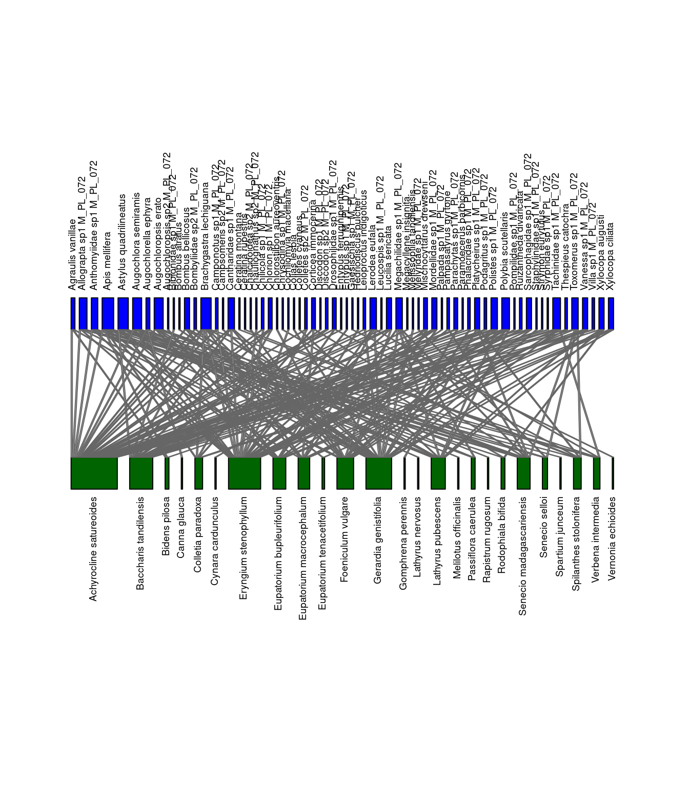
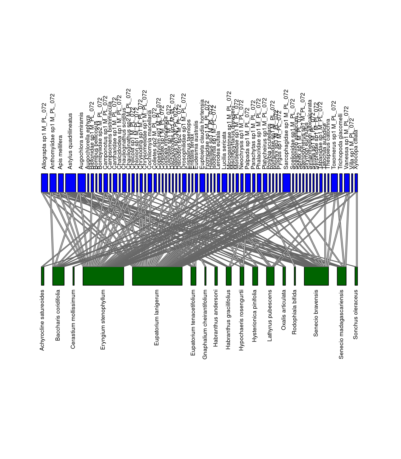 Networks of interactions: M_PL_072_04 (left) and M_PL_072_05 (right). Green represents plants and blue represents pollinators.
Now, let’s calculate β-diversity between M_PL_072_04 and M_PL_072_05 using function betalinkr.
##         S        OS        WN        ST
## 0.5056180 0.4600000 0.8363636 0.3763636
We can also calculate β-diversity between all pairs of networks using function betalinkr_multi.
##              i           j         S        OS        WN        ST
## 1  M_PL_072_01 M_PL_072_02 0.3663366 0.4889868 0.6768802 0.1878934
## 2  M_PL_072_01 M_PL_072_03 0.3721973 0.6390977 0.7762238 0.1371260
## 3  M_PL_072_01 M_PL_072_04 0.4200000 0.5526316 0.8210526 0.2684211
## 4  M_PL_072_01 M_PL_072_05 0.4526316 0.5244755 0.7914110 0.2669355
## 5  M_PL_072_01 M_PL_072_06 0.3500000 0.5475113 0.7245179 0.1770066
## 6  M_PL_072_01 M_PL_072_07 0.3936170 0.5023474 0.7047354 0.2023880
## 7  M_PL_072_01 M_PL_072_08 0.3500000 0.5283843 0.7150396 0.1866553
## 8  M_PL_072_01 M_PL_072_09 0.3516484 0.4881517 0.6625000 0.1743483
## 9  M_PL_072_01 M_PL_072_10 0.4123711 0.6864865 0.8370787 0.1505922
## 10 M_PL_072_01 M_PL_072_11 0.4112150 0.4495413 0.7215777 0.2720364
## 11 M_PL_072_01 M_PL_072_12 0.3365385 0.4375000 0.6538462 0.2163462
## 12 M_PL_072_02 M_PL_072_03 0.3896714 0.6000000 0.7815534 0.1815534
## 13 M_PL_072_02 M_PL_072_04 0.4315789 0.5882353 0.8071625 0.2189272
## 14 M_PL_072_02 M_PL_072_05 0.4555556 0.4876033 0.7993528 0.3117494
## 15 M_PL_072_02 M_PL_072_06 0.4105263 0.5247525 0.7225434 0.1977909
## 16 M_PL_072_02 M_PL_072_07 0.3932584 0.5026455 0.7251462 0.2225007
## 17 M_PL_072_02 M_PL_072_08 0.4000000 0.5098039 0.7237569 0.2139530
## 18 M_PL_072_02 M_PL_072_09 0.3720930 0.5000000 0.7029703 0.2029703
## 19 M_PL_072_02 M_PL_072_10 0.4673913 0.5968992 0.8466077 0.2497084
## 20 M_PL_072_02 M_PL_072_11 0.4215686 0.5390947 0.7294686 0.1903739
## 21 M_PL_072_02 M_PL_072_12 0.3838384 0.4771784 0.6842105 0.2070321
## 22 M_PL_072_03 M_PL_072_04 0.4597156 0.7122302 0.9076212 0.1953910
## 23 M_PL_072_03 M_PL_072_05 0.4427861 0.4968553 0.7889182 0.2920629
## 24 M_PL_072_03 M_PL_072_06 0.4786730 0.7172775 0.8701923 0.1529148
## 25 M_PL_072_03 M_PL_072_07 0.4673367 0.5833333 0.8300971 0.2467638
## 26 M_PL_072_03 M_PL_072_08 0.4502370 0.6701031 0.8518519 0.1817488
## 27 M_PL_072_03 M_PL_072_09 0.4093264 0.6062176 0.7962466 0.1900290
## 28 M_PL_072_03 M_PL_072_10 0.3756098 0.6100000 0.8092910 0.1992910
## 29 M_PL_072_03 M_PL_072_11 0.4577778 0.6082474 0.8429752 0.2347278
## 30 M_PL_072_03 M_PL_072_12 0.4703196 0.5392670 0.8123667 0.2730997
## 31 M_PL_072_04 M_PL_072_05 0.5056180 0.4600000 0.8363636 0.3763636
## 32 M_PL_072_04 M_PL_072_06 0.4042553 0.4345550 0.7057221 0.2711671
## 33 M_PL_072_04 M_PL_072_07 0.3863636 0.4489796 0.7024793 0.2534997
## 34 M_PL_072_04 M_PL_072_08 0.4255319 0.4427861 0.7075718 0.2647857
## 35 M_PL_072_04 M_PL_072_09 0.4705882 0.5474453 0.8086420 0.2611967
## 36 M_PL_072_04 M_PL_072_10 0.4615385 0.6724138 0.8944444 0.2220307
## 37 M_PL_072_04 M_PL_072_11 0.4257426 0.4642857 0.7241379 0.2598522
## 38 M_PL_072_04 M_PL_072_12 0.3877551 0.4628099 0.6904762 0.2276663
## 39 M_PL_072_05 M_PL_072_06 0.4494382 0.5319149 0.7891374 0.2572225
## 40 M_PL_072_05 M_PL_072_07 0.4939759 0.4375000 0.8252427 0.3877427
## 41 M_PL_072_05 M_PL_072_08 0.4494382 0.5338346 0.8115502 0.2777156
## 42 M_PL_072_05 M_PL_072_09 0.3875000 0.4421769 0.6962963 0.2541194
## 43 M_PL_072_05 M_PL_072_10 0.4651163 0.5208333 0.8496732 0.3288399
## 44 M_PL_072_05 M_PL_072_11 0.4687500 0.5460993 0.8320210 0.2859217
## 45 M_PL_072_05 M_PL_072_12 0.4516129 0.4434783 0.8251366 0.3816584
## 46 M_PL_072_06 M_PL_072_07 0.3522727 0.4732143 0.6589595 0.1857453
## 47 M_PL_072_06 M_PL_072_08 0.2978723 0.5489362 0.7103825 0.1614463
## 48 M_PL_072_06 M_PL_072_09 0.4235294 0.5661376 0.7328990 0.1667615
## 49 M_PL_072_06 M_PL_072_10 0.5164835 0.6423841 0.8425656 0.2001815
## 50 M_PL_072_06 M_PL_072_11 0.4059406 0.4732143 0.7177033 0.2444891
## 51 M_PL_072_06 M_PL_072_12 0.4081633 0.4400000 0.6873449 0.2473449
## 52 M_PL_072_07 M_PL_072_08 0.3181818 0.5146444 0.6795580 0.1649137
## 53 M_PL_072_07 M_PL_072_09 0.4303797 0.4520548 0.7359736 0.2839188
## 54 M_PL_072_07 M_PL_072_10 0.4941176 0.6571429 0.8938053 0.2366625
## 55 M_PL_072_07 M_PL_072_11 0.3789474 0.5289575 0.7053140 0.1763565
## 56 M_PL_072_07 M_PL_072_12 0.3152174 0.4000000 0.5639098 0.1639098
## 57 M_PL_072_08 M_PL_072_09 0.4235294 0.4424242 0.7151703 0.2727460
## 58 M_PL_072_08 M_PL_072_10 0.4615385 0.5944056 0.8384401 0.2440345
## 59 M_PL_072_08 M_PL_072_11 0.3564356 0.4981818 0.6820276 0.1838458
## 60 M_PL_072_08 M_PL_072_12 0.3469388 0.5248227 0.6801909 0.1553682
## 61 M_PL_072_09 M_PL_072_10 0.4756098 0.5462185 0.8200000 0.2737815
## 62 M_PL_072_09 M_PL_072_11 0.4782609 0.4319527 0.7440000 0.3120473
## 63 M_PL_072_09 M_PL_072_12 0.4157303 0.4772727 0.7444444 0.2671717
## 64 M_PL_072_10 M_PL_072_11 0.4897959 0.6621622 0.8783455 0.2161833
## 65 M_PL_072_10 M_PL_072_12 0.4842105 0.7226277 0.9040404 0.1814127
## 66 M_PL_072_11 M_PL_072_12 0.3619048 0.4457831 0.6093418 0.1635587
The relative influence of the two components of the total dissimilarity (i.e. \(β_{ST}\) and \(β_{OS}\)) can be expressed in a more intuitive way as fractions \(β_{ST}/β_{WN}\) and \(β_{OS}/β_{WN}\).
# Import dplyr package
library(dplyr)

betadiversity <- betadiversity |>
  mutate(relative_OS = OS/WN,
         relative_ST = ST/WN)

head(betadiversity)
## i j S OS WN ST relative_OS
## 1 M_PL_072_01 M_PL_072_02 0.3663366 0.4889868 0.6768802 0.1878934 0.7224126
## 2 M_PL_072_01 M_PL_072_03 0.3721973 0.6390977 0.7762238 0.1371260 0.8233421
## 3 M_PL_072_01 M_PL_072_04 0.4200000 0.5526316 0.8210526 0.2684211 0.6730769
## 4 M_PL_072_01 M_PL_072_05 0.4526316 0.5244755 0.7914110 0.2669355 0.6627094
## 5 M_PL_072_01 M_PL_072_06 0.3500000 0.5475113 0.7245179 0.1770066 0.7556905
## 6 M_PL_072_01 M_PL_072_07 0.3936170 0.5023474 0.7047354 0.2023880 0.7128171
## relative_ST
## 1 0.2775874
## 2 0.1766579
## 3 0.3269231
## 4 0.3372906
## 5 0.2443095
## 6 0.2871829
Finally, let’s calculate the interaction β-diversity between the networks and the metaweb.
A metaweb is the regional pool of species and their potential interactions. A local network is a realization from a regional metaweb.
Understanding the interaction β-diversity between local networks and the metaweb allows us to characterize the diversity of interactions in space, which is the first step in developing a predictive theory of spatial network ecology.
We need to create the metaweb and join the metaweb with the rest of the networks.
# Import abind package
library(abind)

# Create a metaweb by summing all interactions across all networks
metaweb <- as.array(rowSums(network_array, dims=2), dim=3,
                    dimnames=list("species1", "species2", "network_name"))

# Combine with local networks
network_array <- abind(network_array, metaweb)

# Set network_name to "metaweb"
dimnames(network_array)[[3]][13] = "metaweb"

# Check that network_array contains all local networks and the metaweb
dimnames(network_array)[[3]]
## [1] "M_PL_072_01" "M_PL_072_02" "M_PL_072_03" "M_PL_072_04" "M_PL_072_05"
## [6] "M_PL_072_06" "M_PL_072_07" "M_PL_072_08" "M_PL_072_09" "M_PL_072_10"
## [11] "M_PL_072_11" "M_PL_072_12" "metaweb"Now, in the network_array object, we have the local networks and the metaweb. β-diversity can now be recalculated using the function betalinkr_multi, just like we did it for all the sites.
6.4 Interpretation of R output
S - dissimilarity in species composition \(β_{S}\)
- \(β_{S}=0\): all species co-occur in both networks
- \(β_{S}=1\): no common species in two networks
OS - dissimilarity due to rewiring \(β_{OS}\)
- \(β_{OS}=0\): all links between species that co-occur in the two networks are found in the two networks
- \(β_{OS}=1\): no common links between species that co-occur in the two networks are found in the two networks
WN - dissimilarity of interactions \(β_{WN}\)
- \(β_{WN}=0\): every link between species is found in both networks
- \(β_{WN}=1\): no common links in two networks
ST - dissimilarity due to species turnover \(β_{ST}\)
- \(β_{ST}=0\): no links found between species that occur in one network but not in the other
- \(β_{ST}=1\): every link found in one network is not found in the other because the species involved did not co-occur
6.5 Exercises
We have learned how to evaluate the interaction β-diversity on a network dataset. Now, it’s your turn to explore interaction β-diversity among the 12 communities from the Argentinian ‘sierras’, and relate it to the geographical distance between them. Follow these steps:
Step 1
Download the 12 networks from the Web of Life (M_PL_072_XX).
Hint: see the example code above
Step 2
Calculate the β-diversity for the 12 local networks.
Hint: see the example code above
Step 3
Download the network data for the 12 networks from the Web of Life.
Hint: Use the following code to download data for all networks in the Web of Life, and select relevant networks and information:
# Download information for all networks
all_network_info <- read.csv("https://www.web-of-life.es/get_network_info.php")

# Select relevant networks and information
network_info <- all_network_info |>
  filter(network_name %in% c("M_PL_072_01","M_PL_072_02","M_PL_072_03",
                             "M_PL_072_04","M_PL_072_05","M_PL_072_06",
                             "M_PL_072_07","M_PL_072_08","M_PL_072_09",
                             "M_PL_072_10","M_PL_072_11","M_PL_072_12")) |>
  select(network_name, latitude, longitude)
Step 4
Calculate the geographical distance between the 12 communities using their coordinates, and store it in a dataframe.
Hint: Use the function distm from package geosphere, and the following code to calculate distances between sites:
# Import geosphere and reshape2 packages
library(geosphere)
library(reshape2)

# Create distance matrix
distance_matrix <- distm(network_info[,c("longitude","latitude")], fun=distHaversine)
colnames(distance_matrix) <- network_info$network_name
rownames(distance_matrix) <- network_info$network_name

# Transform the distance matrix into dataframe
distance_data <- distance_matrix |>
  melt() |>
  dplyr::rename(i=Var1, j=Var2, distance=value)
Step 5
Join the betadiversity and site distance dataframes.
Hint: use function left_join from dplyr to join the two data frames by columns i and j.
Step 6
Plot the relationship between geographical distance and the different components of interaction β-diversity (\(β_{WN}\), \(β_{ST}/β_{WN}\) and \(β_{OS}/β_{WN}\)).
Hint: you can use the function ggplot from package ggplot2.
Questions
Please answer the following questions in your RScripts (use # at the start of each line):
Q1: What is the relationship between geographical distance and interaction β-diversity?
Q2: Is interaction β-diversity mainly explained by the species turnover or by the interaction rewiring?
Q3: What could be the implications of your observations for conservation?
Q4: Throughout this course, you also learned that we can compare the networks using the topology metrics of networks (e.g. nestedness, modularity, connectance). What is the difference between using interaction β-diversity and the other metrics? What new information does β-diversity offer?
Bonus exercise
Explore the differences in β-diversity of the 12 sites with the metaweb.
6.6 Solutions
Step 1 Download the 12 networks from the Web of Life (M_PL_072_XX).
# Define networks to be downloaded
network_names <- list("M_PL_072_01","M_PL_072_02","M_PL_072_03",
                      "M_PL_072_04","M_PL_072_05","M_PL_072_06",
                      "M_PL_072_07","M_PL_072_08","M_PL_072_09",
                      "M_PL_072_10","M_PL_072_11","M_PL_072_12")

# Download all networks and store as a single dataframe
network_data <- NULL
for (nw_name in network_names){
  json_url <- paste0("https://www.web-of-life.es/get_networks.php?network_name=",nw_name)
  new_nw_rows <- jsonlite::fromJSON(json_url)
  network_data <- rbind(network_data, new_nw_rows)
}

# Convert connection strength to numeric values
network_data$connection_strength <- as.numeric(network_data$connection_strength)
Step 2
Calculate the β-diversity for the 12 local networks.
# Convert dataframe to 3D array
network_array <- frame2webs(network_data,
                            varnames=c("species1", "species2",
                                       "network_name", "connection_strength"),
                            type.out="array")

# Calculate beta-diversity
betadiversity <- betalinkr_multi(network_array, partitioning="poisot", binary=TRUE)

# Calculate relative contributions of OS and ST
betadiversity <- betadiversity |>
  mutate(relative_OS = OS/WN,
         relative_ST = ST/WN)


head(betadiversity)
## i j S OS WN ST relative_OS
## 1 M_PL_072_01 M_PL_072_02 0.3663366 0.4889868 0.6768802 0.1878934 0.7224126
## 2 M_PL_072_01 M_PL_072_03 0.3721973 0.6390977 0.7762238 0.1371260 0.8233421
## 3 M_PL_072_01 M_PL_072_04 0.4200000 0.5526316 0.8210526 0.2684211 0.6730769
## 4 M_PL_072_01 M_PL_072_05 0.4526316 0.5244755 0.7914110 0.2669355 0.6627094
## 5 M_PL_072_01 M_PL_072_06 0.3500000 0.5475113 0.7245179 0.1770066 0.7556905
## 6 M_PL_072_01 M_PL_072_07 0.3936170 0.5023474 0.7047354 0.2023880 0.7128171
## relative_ST
## 1 0.2775874
## 2 0.1766579
## 3 0.3269231
## 4 0.3372906
## 5 0.2443095
## 6 0.2871829
Step 3
Download the network data for the 12 networks from the Web of Life.
# Download network information
all_network_info <- read.csv("https://www.web-of-life.es/get_network_info.php")

# Select relevant networks and information
network_info <- all_network_info |>
  filter(network_name %in% c("M_PL_072_01","M_PL_072_02","M_PL_072_03",
                             "M_PL_072_04","M_PL_072_05","M_PL_072_06",
                             "M_PL_072_07","M_PL_072_08","M_PL_072_09",
                             "M_PL_072_10","M_PL_072_11","M_PL_072_12")) |>
  select(network_name, latitude, longitude)
Step 4
Calculate the geographical distance between the 12 communities using their coordinates, and store it in a dataframe.
# Import geosphere and reshape2 packages
library(geosphere)
library(reshape2)

# Create distance matrix
distance_matrix <- distm(network_info[,c("longitude","latitude")], fun=distHaversine)
colnames(distance_matrix) = rownames(distance_matrix) = network_info$network_name

# transform the distance matrix into dataframe
distance_data <- distance_matrix |>
  melt() |>
  dplyr::rename(i=Var1, j=Var2, distance=value)

head(distance_data)
## i j distance
## 1 M_PL_072_01 M_PL_072_01 0.000
## 2 M_PL_072_02 M_PL_072_01 16008.988
## 3 M_PL_072_03 M_PL_072_01 13524.212
## 4 M_PL_072_04 M_PL_072_01 45657.806
## 5 M_PL_072_05 M_PL_072_01 13275.179
## 6 M_PL_072_06 M_PL_072_01 9289.067
Step 5
Join the betadiversity and site distance dataframes.
Step 6
Plot the relationship between geographical distance and the different components of interaction β-diversity (\(β_{WN}\), \(β_{ST}/β_{WN}\) and \(β_{OS}/β_{WN}\)).
# transform data for plotting
betadiv_WN <- betadiversity |>
  mutate(beta_diversity = "WN", beta_value = WN) |>
  select(i, j, distance, beta_diversity, beta_value)
betadiv_OS <- betadiversity |>
  mutate(beta_diversity = "OS/WN", beta_value = OS/WN) |>
  select(i, j, distance, beta_diversity, beta_value)
betadiv_ST <- betadiversity |>
  mutate(beta_diversity = "ST/WN", beta_value = ST/WN) |>
  select(i, j, distance, beta_diversity, beta_value)
betadiv <- rbind(betadiv_WN, betadiv_OS, betadiv_ST)

# plot betadiversity vs distance
ggplot(data=betadiv, aes(x=distance, y=beta_value, col=beta_diversity)) +
  geom_point() +
  geom_smooth(method=lm) +
  ylim(c(0,1))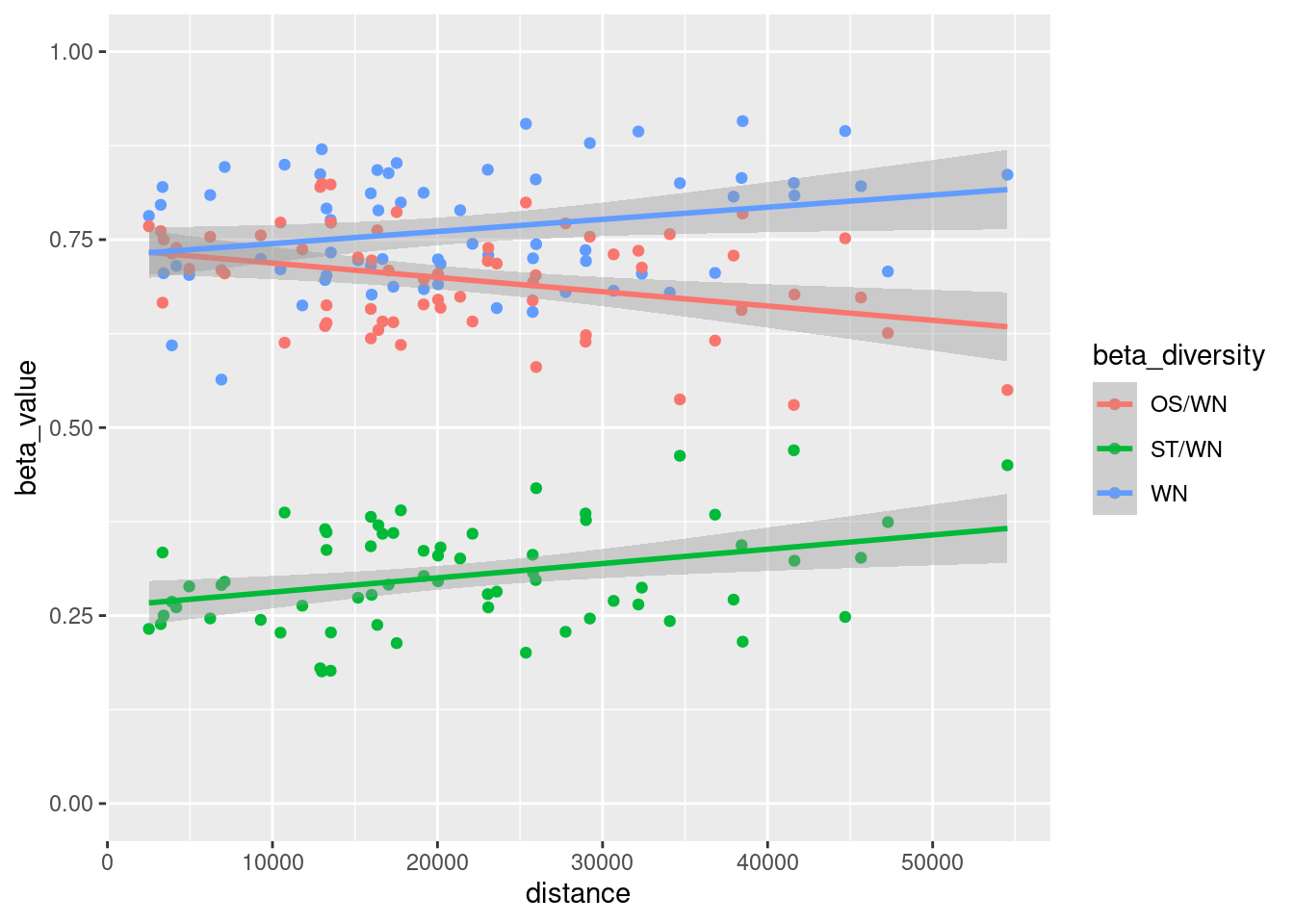
Questions
Please answer the following questions in your RScripts (use # at the start of
each line):
Q1: What is the relationship between geographical distance and interaction β-diversity?
A1: The relationship between geographical distance and interaction β-diversity is often positive, meaning that as geographical distance increases interaction β-diversity tends to increase.
Q2: Is interaction β-diversity mainly explained by the species turnover or by the interaction rewiring?
A2: While species turnover is often the main driver of interaction β-diversity, interaction rewiring can play a significant role, particularly at local scales and in flexible interaction networks. Our plot also suggests that interaction rewiring contributes more at shorter distances, whereas species turnover becomes increasingly dominant in explaining β-diversity as distance increases. The balance between these two mechanisms depends on factors such as species dispersal, ecological specialization, and environmental heterogeneity.
Q3: What could be the implications of your observations for conservation?
A3: Species turnover tends to increase with geographical distance, which highlights the need to conserve multiple habitats across large areas. In contrast, interaction rewiring is more significant at smaller distances, where species adapt their interactions. Conservation strategies should address both processes by ensuring habitat connectivity to minimize species loss over distance and maintaining conditions that allow species to flexibly adjust their ecological relationships.
Q4: Throughout this course, you also learned that we can compare the networks using the topology metrics of networks (e.g. nestedness, modularity, connectance). What is the difference between using interaction β-diversity and the other metrics? What new information does β-diversity offer?
A4: Topology metrics such as nestedness, modularity, and connectance describe the structure and connectivity of networks. In contrast, interaction β-diversity measures dissimilarity in species interactions across environments or spatial scales. While topology metrics focus on static network properties, β-diversity reveals how ecological relationships—such as mutualistic interactions between species—shift under different conditions, offering a dynamic view of community changes that structural metrics might overlook.
Bonus exercise
Explore the differences in β-diversity of the 12 sites with the metaweb.
# Create a metaweb by summing all interactions across all networks
metaweb <- as.array(rowSums(network_array, dims=2), dim=3,
                    dimnames=list("species1", "species2", "network_name"))

# Combine with local networks
network_array <- abind(network_array, metaweb)

# Set network_name to "metaweb"
dimnames(network_array)[[3]][13] = "metaweb"

# Check that network_array contains all local networks and the metaweb
dimnames(network_array)[[3]]
## [1] "M_PL_072_01" "M_PL_072_02" "M_PL_072_03" "M_PL_072_04" "M_PL_072_05"
## [6] "M_PL_072_06" "M_PL_072_07" "M_PL_072_08" "M_PL_072_09" "M_PL_072_10"
## [11] "M_PL_072_11" "M_PL_072_12" "metaweb"# Calculate beta-diversity
betadiversity_meta <- betalinkr_multi(network_array,
partitioning="poisot", binary=TRUE)
# Calculate relative contributions of OS and ST
betadiversity_meta <- betadiversity_meta |>
mutate(relative_OS = OS/WN,
relative_ST = ST/WN)
# transform data for plotting
betadiv_WN_meta <- betadiversity_meta |>
mutate(beta_diversity = "WN", beta_value = WN) |>
select(i, j, beta_diversity, beta_value)
betadiv_OS_meta <- betadiversity_meta |>
mutate(beta_diversity = "OS/WN", beta_value = OS/WN) |>
select(i, j, beta_diversity, beta_value)
betadiv_ST_meta <- betadiversity_meta |>
mutate(beta_diversity = "ST/WN", beta_value = ST/WN) |>
select(i, j, beta_diversity, beta_value)
betadiv_meta <- rbind(betadiv_WN_meta, betadiv_OS_meta, betadiv_ST_meta)
# plot
ggplot(data=filter(betadiv_meta, j=="metaweb", beta_diversity=="WN"),
aes(x=i, y=beta_value)) +
geom_bar(stat="identity") +
lims(y=c(0,1)) +
theme(axis.text.x = element_text(angle = 90, vjust = 0.5, hjust=1)) +
xlab("") + ylab("beta value")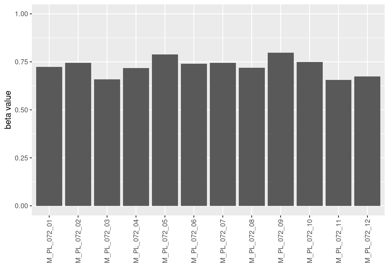
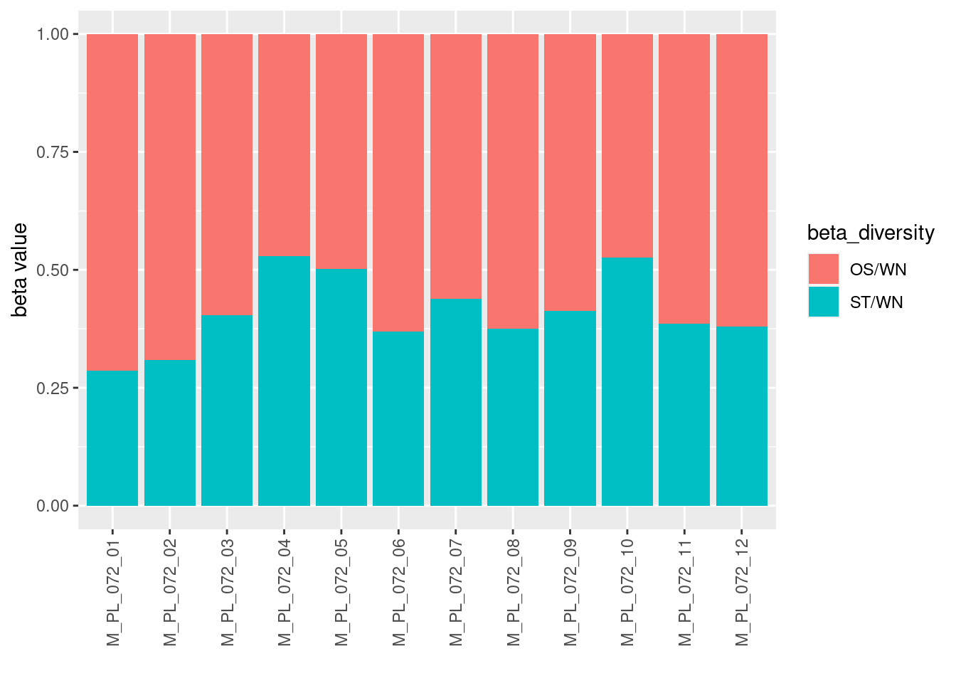
ggplot(data=filter(betadiv_meta, j=="metaweb", beta_diversity!="WN"),
       aes(x=i, y=beta_value, fill=beta_diversity)) +
  geom_bar(stat="identity") +
  theme(axis.text.x = element_text(angle = 90, vjust = 0.5, hjust=1)) +
  xlab("") + ylab("beta value")