2 Measuring modularity
Marilia Palumbo Gaiarsa & Daniel Wechsler
session 18/03/2022
2.1 Plotting networks
For this exercise we will be using the igraph library.
# Import the required libraries
library(igraph)
library(dplyr)
library(rjson)
library(formattable)
Now we will download a network from Web of life and create a bipartite igraph object from it (see session Toolkit for network analysis):
# download the M_PA_002 network from the web-of-life API
json_url <- paste0("https://www.web-of-life.es/get_networks.php?network_name=M_PA_002")
M_PA_002_nw <- jsonlite::fromJSON(json_url)

# select the 3 relevant columns and create the igraph object
graph_staGen <- M_PA_002_nw %>% select(species1, species2, connection_strength) %>%
  graph_from_data_frame(directed = FALSE)

# Add the "type" attribute to the vertices to turn the object graph_staGen into a bipartite graph
V(graph_staGen)$type <- bipartite_mapping(graph_staGen)$type

graph_staGen #checking
## IGRAPH 4834f60 UN-B 10 13 --
## + attr: name (v/c), type (v/l), connection_strength (e/c)
## + edges from 4834f60 (vertex names):
## [1] Cecropia ficifolia --Azteca xanthochroa
## [2] Cecropia ficifolia --Camponotus balzani
## [3] Cecropia membranacea --Azteca ovaticeps
## [4] Cecropia membranacea --Azteca xanthochroa
## [5] Cecropia membranacea --Camponotus balzani
## [6] Cecropia engleriana --Azteca ovaticeps
## [7] Cecropia engleriana --Azteca xanthochroa
## [8] Cecropia polystachya --Azteca ovaticeps
## + ... omitted several edgesYou can access object information using $:
V(graph_staGen) # to see the vertices (nodes) names = species ## + 10/10 vertices, named, from 4834f60:
## [1] Cecropia ficifolia Cecropia membranacea Cecropia engleriana
## [4] Cecropia polystachya Cecropia tessmannii Cecropia sp1 M_PA_002
## [7] Azteca xanthochroa Camponotus balzani Azteca ovaticeps
## [10] Pachycondyla luteolaE(graph_staGen) # to see the edges (pairwise interactions)## + 13/13 edges from 4834f60 (vertex names):
## [1] Cecropia ficifolia --Azteca xanthochroa
## [2] Cecropia ficifolia --Camponotus balzani
## [3] Cecropia membranacea --Azteca ovaticeps
## [4] Cecropia membranacea --Azteca xanthochroa
## [5] Cecropia membranacea --Camponotus balzani
## [6] Cecropia engleriana --Azteca ovaticeps
## [7] Cecropia engleriana --Azteca xanthochroa
## [8] Cecropia polystachya --Azteca ovaticeps
## [9] Cecropia polystachya --Azteca xanthochroa
## [10] Cecropia polystachya --Camponotus balzani
## + ... omitted several edgesLet’s plot our Graph object. igraph provides several layouts to plot graphs. Some of the available layouts are:
- layout_in_circle
- layout_randomly
- layout_with_fr.
For more options to customize the plot (e.g. edge width) see for example: https://igraph.org/r/doc/plot.common.html or https://www.r-graph-gallery.com/248-igraph-plotting-parameters/. Since this is a bipartite nwtroks, let’s use the bipartite layout.
plot(graph_staGen,
     layout=layout_as_bipartite,
     vertex.color="azure",
     margin=0.0)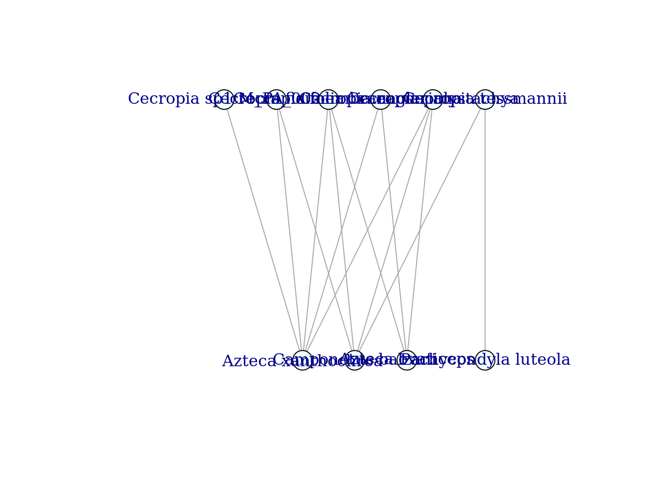
2.2 Computing Modularity
Now that we have the igraph object let’s compute modularity. Sometimes the user may have a pre-defined node partitioning. If that is the case, we can manually define the modules if you already know which module which species belongs to.
# Manually define partitioning
membership = c(1,2,2,2,3,2,1,3,2,2)
# Compute modularity of partitioning
Q <- modularity(graph_staGen, membership)
Q
## [1] 0.00887574We can also color the nodes according to the modules and plot the graph
# Color the nodes according to the modules
colbar <- rainbow(max(membership))
V(graph_staGen)$color <- colbar[membership]

# Plot the graph
plot(graph_staGen, layout=layout_with_fr, margin=0.0)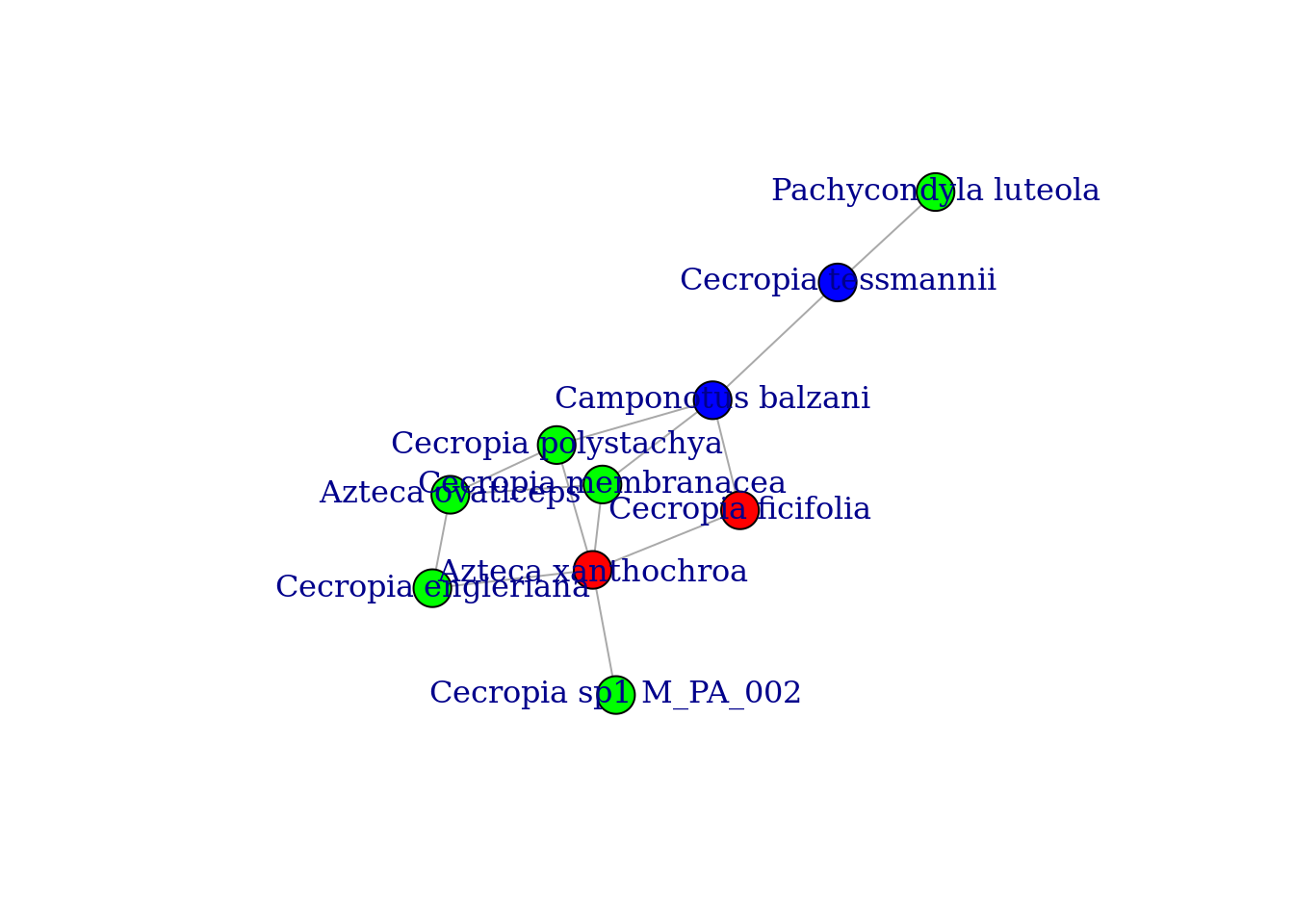
2.3 Computing Detection
Some community detection algorithms available in igraph are:
- cluster_label_prop
- cluster_edge_betweenness
- cluster_fast_greedy
- cluster_leading_eigen
- cluster_optimal (SLOW!!)
Instead of having a predetermined idea of to which module each species belongs to, it is much more common to find the best partitioning of the nodes using one of the available community detection algorithms. Let us use the fast greedy algorithm:
modules <- cluster_fast_greedy(graph_staGen)
modules$membership # looking at the result
## [1] 2 1 1 1 2 1 1 2 1 2Let’s get the modularity of the best partitioning.
M <- modularity(modules)
M
## [1] 0.2218935Again, we can now color the nodes of our graph according the module they belong to.
colbar <- rainbow(max(modules$membership))
V(graph_staGen)$color <- colbar[modules$membership]

plot(graph_staGen,
     layout=layout_with_fr,
     vertex.size=12,
     margin=0.0)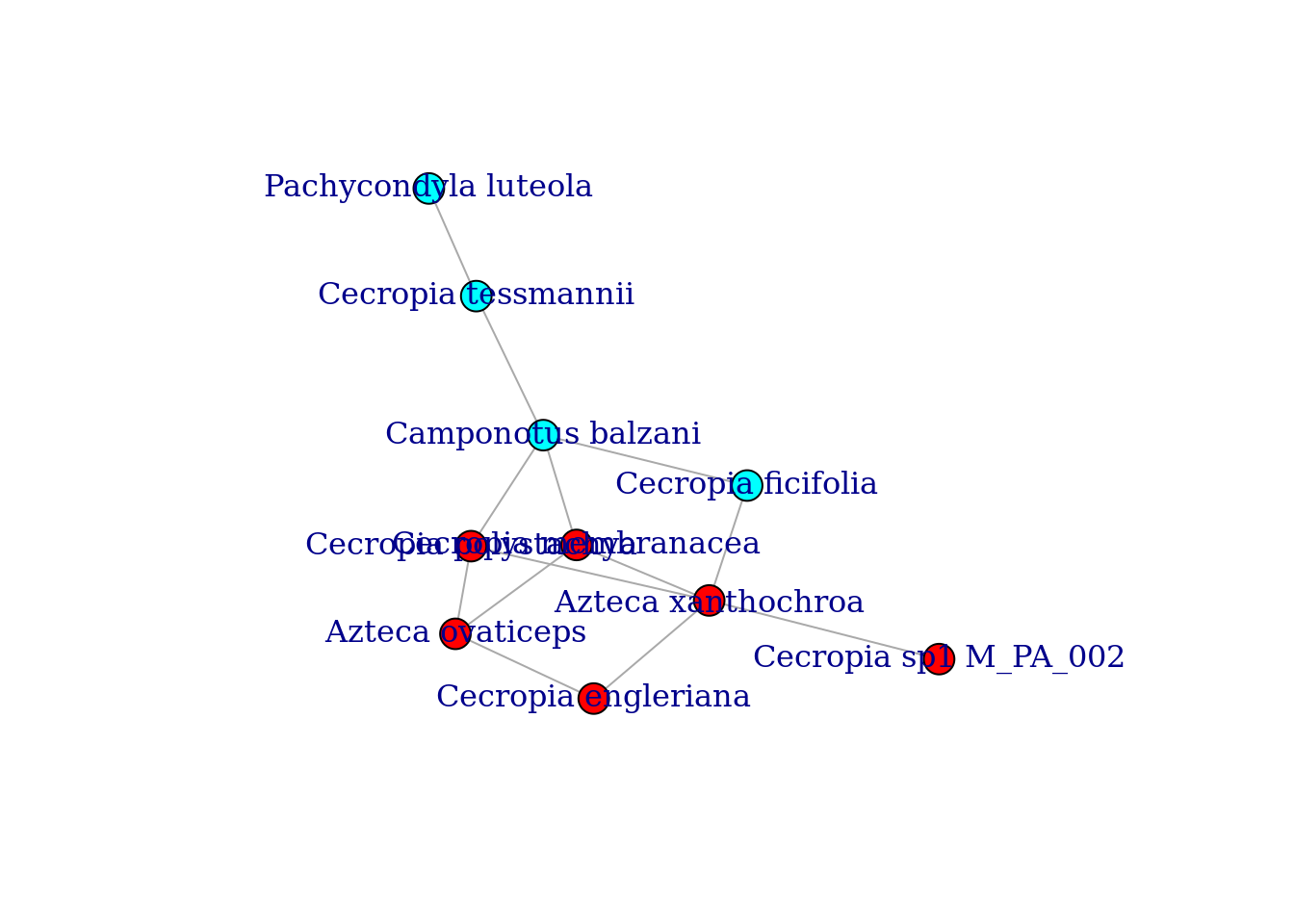
This layout makes much more sense!
2.4 Exercises
Remember to follow the instructions provided in the template.R on the first day of class. For the exercises on paper, please take a picture of your work and upload it to the server or email it to me marilia.gaiarsa@ieu.uzh.ch.
2.4.0.1 Question 1
For the graph drawn below do the following (on paper):
- Compute for each node its degree.
- Compute the adjacency matrix.
B <- matrix(c(0,0,1,0,1,0,0,0,0,1,1,0,1,0,0,1,1,1,0,1,1,0,0,1,1,1,1,0,0,1,0,0,1,1,1,0),nrow=6,ncol=6)
graph <- graph_from_adjacency_matrix(B,mode="undirected")

# PLot network using bipartite layout
plot(graph,
     vertex.size = 8,
     vertex.label.color = 'black',
     vertex.color = 'orange',
     margin = 0.0,
     asp = 0.5)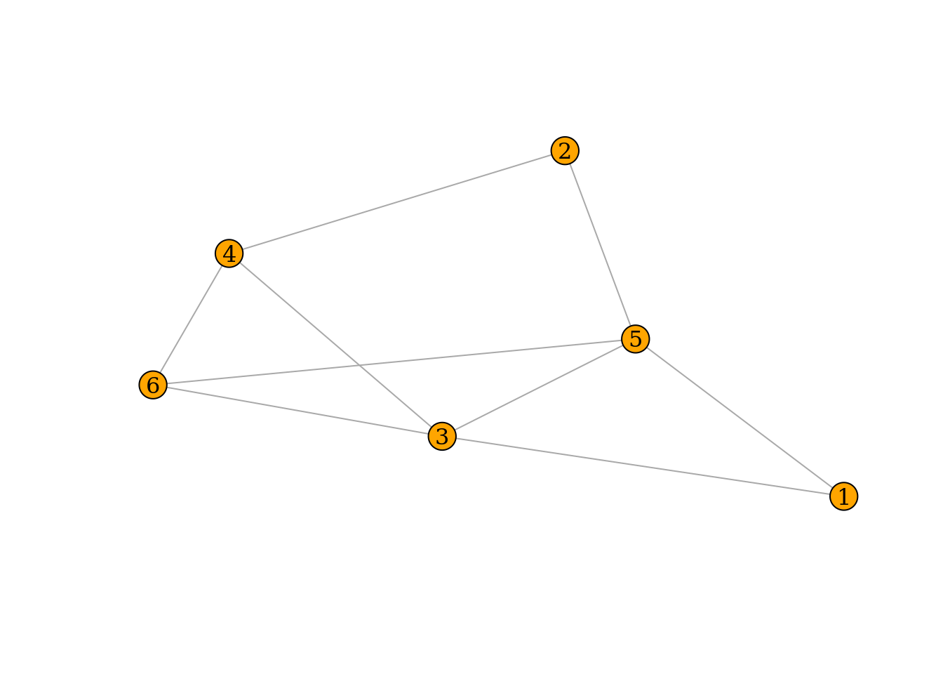
2.4.0.2 Question 2
Draw the graph represented by the following adjacency matrix (on paper):
\[ \\A = \begin{bmatrix} 0 & 0 & 1 & 0 & 1 \\ 0 & 0 & 0 & 1 & 1 \\ 1 & 0 & 0 & 0 & 0 \\ 0 & 1 & 0 & 0 & 1 \\ 1 & 1 & 0 & 1 & 0 \\ \end{bmatrix} \]
2.4.0.3 Question 3
The node colors of the graph below represent a partitioning of the nodes into three modules.
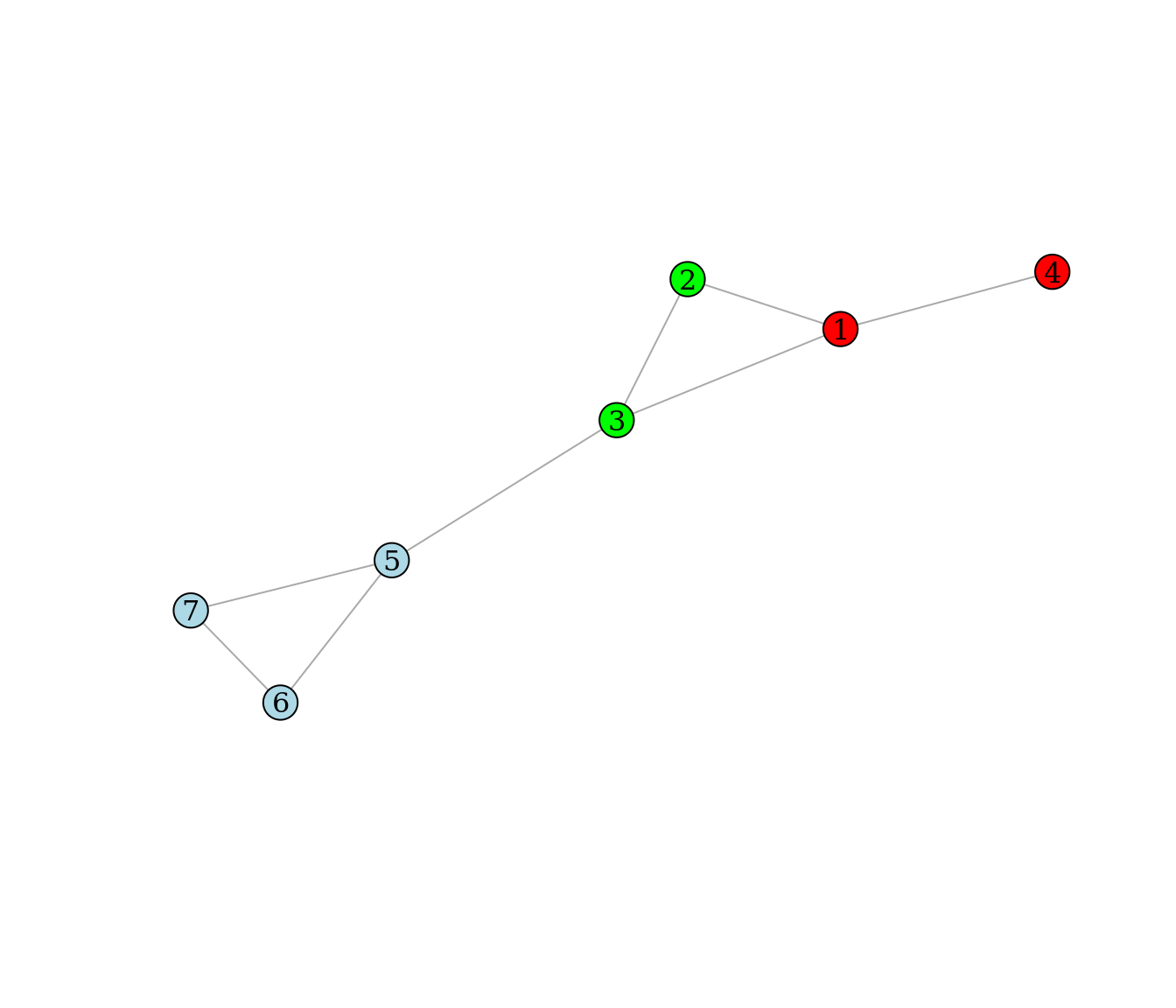
Use the formula from the slides to compute the modularity Q of the partitioning (on paper).
Check your answer using R.
Do you think the given node partitioning is the best, i.e. it optimizes Q (argue)?
2.4.0.4 Question 4
Using the code to download files from the Web of Life database, download the network named M_SD_001 and:
Use the community detection algorithm cluster_louvain to compute the “optimal” node partitioning (modules) for the network.
Compute the modularity M.
Plot both networks. Color the nodes according to the modules and try to find the layout that best shows the communities.