11 Socio-ecological networks
Rodrigo Cámara-Leret
session 6/04/2022
11.1 Indigenous knowledge networks
Today we will apply some of the network analyses used in the paper: R. Cámara-Leret, M. Fortuna & J. Bascompte (2019). Indigenous knowledge networks in the face of global change. PNAS: 116 (20) 9913-9918.
In contrast with previous exercises, today each network will be an indigenous knowledge network and we will use a dataset of 57 indigenous communities of South America. We can depict indigenous knowledge networks as bipartite graphs: nodes on one set represent plant species (in this case, of the palm family Arecaceae), nodes on the other set represent plant services, and a link connecting a plant species to a service indicates that the indigenous community knows that the plant provides them that service.
Let’s begin by loading all the R packages we need for today:
library(igraph)
library(betalink)
library(bipartite)
library(calibrate)
Now let’s list the networks we will be working with today.There should be 57 csv files, one for each community. Note: the aggregated data is also available in Table S4 of Cámara-Leret et al 2019.
list.files("~/ecological_networks_2022/downloads/Data/04-06_socio-ecological_networks/")## [1] "Aguacate.csv" "AltoIvon.csv"
## [3] "Angostura.csv" "Aviacion.csv"
## [5] "BuenaVista.csv" "Camaritagua.csv"
## [7] "CentroProvidencia.csv" "Chiguilpe.csv"
## [9] "community_classification.csv" "Correo.csv"
## [11] "Curare.csv" "CusuChico.csv"
## [13] "Dureno.csv" "ElChino.csv"
## [15] "Illipanayuyo.csv" "Irimo.csv"
## [17] "Juisanoy.csv" "Kapawi.csv"
## [19] "Kusutkau.csv" "LamasWayku.csv"
## [21] "Mayo.csv" "Mindo.csv"
## [23] "Motacuzal.csv" "Munaypata.csv"
## [25] "Nanegalito.csv" "networks.RData"
## [27] "NuevaSamaria.csv" "NuevoProgreso.csv"
## [29] "Octubre.csv" "Pacuya.csv"
## [31] "PalmaReal.csv" "Peripa.csv"
## [33] "Pucasucho.csv" "PuertoPervel.csv"
## [35] "PuertoQuito.csv" "PuertoYaminahua.csv"
## [37] "Sanandita.csv" "SanAntonio.csv"
## [39] "SanBenito.csv" "SanIsidro.csv"
## [41] "SanMartin.csv" "SanMartinDeAmacayacu.csv"
## [43] "SanSilvestre.csv" "SantaAna.csv"
## [45] "SantaMaria.csv" "SantaRosa.csv"
## [47] "SantaRosaDeMaravilla.csv" "Santiago.csv"
## [49] "SantoDomingoBolivia.csv" "Secejsama.csv"
## [51] "Sibundoy.csv" "TresArroyos.csv"
## [53] "UnionProgreso.csv" "Villanueva.csv"
## [55] "VillaSantiago.csv" "Wayusentsa.csv"
## [57] "Yamayakat.csv" "Yucuna.csv"
## [59] "Zabalo.csv"Now we READ one indigenous knowledge network (one community). Fieldwork note: this community is of the Embera indigenous peoples; it is relative isolated in the Pacific lowlands of Colombia (in the Chocó biodiversity hotspot) and is only accessible by canoe.

Aguacate <- read.table("~/ecological_networks_2022/downloads/Data/04-06_socio-ecological_networks/Aguacate.csv", sep=",", header=TRUE, row.names=1)
str(Aguacate)
## 'data.frame': 33 obs. of 54 variables:
## $ Bract_Cultural_Clothes.and.accessories : int 0 0 0 0 0 0 0 0 0 0 ...
## $ Bract_Utensils...tools_Domestic.utensils : int 0 0 0 0 0 0 0 0 0 0 ...
## $ Bract_Utensils...tools_Labour.tools : int 0 0 0 0 0 0 0 0 0 0 ...
## $ Bract_Utensils...tools_Other : int 0 0 0 0 0 0 0 0 0 0 ...
## $ Entire.leaf_Construction_Thatch : int 1 0 1 0 1 0 0 0 0 0 ...
## $ Entire.leaf_Cultural_Ritual : int 1 0 0 0 1 0 0 0 0 0 ...
## $ Entire.leaf_Fuel_Lighting : int 0 0 0 1 0 0 0 0 0 0 ...
## $ Entire.leaf_Medicinal...veterinary_Blood.and.Cardio.vascular.system: int 0 0 0 0 0 0 0 0 0 0 ...
## $ Entire.leaf_Utensils...tools_Domestic.utensils : int 0 0 1 0 0 0 0 0 0 0 ...
## $ Entire.leaf_Utensils...tools_Hunting.and.fishing : int 0 0 0 0 0 0 0 0 0 0 ...
## $ Entire.leaf_Utensils...tools_Wrappers : int 0 0 1 0 0 0 0 0 0 0 ...
## $ Fruit_Animal.food_Fodder : int 0 0 1 1 0 0 0 0 0 0 ...
## $ Fruit_Animal.food_Wildlife.attractant : int 0 0 0 1 0 0 0 0 0 0 ...
## $ Fruit_Cultural_Personal.adornment : int 0 0 0 1 1 1 0 0 0 0 ...
## $ Fruit_Cultural_Recreational : int 0 0 0 1 0 0 0 0 0 0 ...
## $ Fruit_Human.food_Beverages : int 1 0 1 0 0 0 1 1 1 0 ...
## $ Fruit_Human.food_Food : int 1 0 0 1 0 0 1 1 1 0 ...
## $ Fruit_Human.food_Food.additives : int 0 0 0 1 0 0 0 0 0 0 ...
## $ Fruit_Human.food_Oils : int 1 0 0 0 0 0 0 1 0 0 ...
## $ Fruit_Medicinal...veterinary_Reproductive.system.and.sex.health : int 0 0 0 0 0 0 0 0 1 0 ...
## $ Inflorescence_Cultural_Recreational : int 1 0 0 0 0 0 0 0 0 0 ...
## $ Leaf.sheath_Cultural_Recreational : int 0 0 0 0 0 0 0 0 0 0 ...
## $ Leaf.sheath_Utensils...tools_Other : int 0 0 0 0 0 0 0 0 0 0 ...
## $ Palm.heart_Human.food_Food : int 1 0 1 1 1 1 1 0 0 0 ...
## $ Petiole_Utensils...tools_Domestic.utensils : int 1 0 1 0 0 0 0 0 0 0 ...
## $ Petiole_Utensils...tools_Hunting.and.fishing : int 0 0 0 0 0 0 0 0 0 1 ...
## $ Root_Cultural_Ritual : int 0 0 0 0 0 0 0 0 0 0 ...
## $ Root_Utensils...tools_Domestic.utensils : int 0 0 0 0 0 0 0 0 0 0 ...
## $ Seed_Cultural_Personal.adornment : int 0 0 0 0 0 0 0 0 0 0 ...
## $ Seed_Cultural_Recreational : int 0 0 0 0 0 0 0 0 0 0 ...
## $ Seed_Human.food_Beverages : int 0 0 0 1 1 0 0 0 0 0 ...
## $ Seed_Human.food_Food : int 0 0 1 1 1 1 1 1 1 1 ...
## $ Seed_Medicinal...veterinary_Not.specified.at.all : int 0 0 0 0 0 0 0 0 0 0 ...
## $ Spear.leaf_Cultural_Clothes.and.accessories : int 0 0 0 1 1 0 0 0 0 0 ...
## $ Spear.leaf_Cultural_Personal.adornment : int 0 0 0 1 0 0 0 0 0 0 ...
## $ Spear.leaf_Cultural_Recreational : int 0 0 0 0 1 1 0 0 0 0 ...
## $ Spear.leaf_Cultural_Ritual : int 1 0 0 1 1 0 0 0 0 0 ...
## $ Spear.leaf_Utensils...tools_Domestic.utensils : int 0 0 1 1 1 0 0 0 0 0 ...
## $ Spear.leaf_Utensils...tools_Rope : int 0 0 0 0 0 0 0 0 0 0 ...
## $ Spines_Medicinal...veterinary_Skin.and.subcutaneous.tissue : int 0 0 0 1 0 0 1 1 1 1 ...
## $ Stem_Construction_Houses : int 1 0 0 1 0 0 0 0 0 0 ...
## $ Stem_Construction_Thatch : int 0 0 0 0 0 0 0 0 0 0 ...
## $ Stem_Construction_Transportation : int 0 0 0 0 0 0 0 0 0 0 ...
## $ Stem_Cultural_Clothes.and.accessories : int 0 0 0 0 0 0 0 0 0 0 ...
## $ Stem_Cultural_Recreational : int 0 0 0 0 0 0 0 0 0 0 ...
## $ Stem_Cultural_Ritual : int 0 0 0 1 0 0 0 0 0 0 ...
## $ Stem_Environmental_Fences : int 0 0 0 0 0 0 0 0 0 0 ...
## $ Stem_Fuel_Firewood : int 1 0 1 1 0 0 0 0 0 0 ...
## $ Stem_Medicinal...veterinary_Skin.and.subcutaneous.tissue : int 0 0 0 0 0 0 0 0 0 0 ...
## $ Stem_Other_Miscellaneous : int 1 0 0 0 0 0 1 0 0 0 ...
## $ Stem_Utensils...tools_Domestic.utensils : int 0 0 0 0 0 0 0 0 0 0 ...
## $ Stem_Utensils...tools_Hunting.and.fishing : int 1 0 0 1 0 0 1 1 1 1 ...
## $ Stem_Utensils...tools_Labour.tools : int 0 0 0 1 0 0 0 0 0 0 ...
## $ Stem_Utensils...tools_Rope : int 0 0 0 0 0 0 0 0 0 0 ...Our network is read as a data frame, made up of rows (species) and columns (plant services). How many plant species and plant services are there in this indigenous knowledge network?
# Number of plant species
nrow(Aguacate)
## [1] 33# Number of plant services
ncol(Aguacate)## [1] 54Let’s continue and read all other indigenous knowledge networks.
AltoIvon <- read.table("~/ecological_networks_2022/downloads/Data/04-06_socio-ecological_networks/AltoIvon.csv", sep=",", header=TRUE, row.names=1)
Angostura <- read.table("~/ecological_networks_2022/downloads/Data/04-06_socio-ecological_networks/Angostura.csv", sep=",", header=TRUE, row.names=1)
Aviacion <- read.table("~/ecological_networks_2022/downloads/Data/04-06_socio-ecological_networks/Aviacion.csv", sep=",", header=TRUE, row.names=1)
BuenaVista <- read.table("~/ecological_networks_2022/downloads/Data/04-06_socio-ecological_networks/BuenaVista.csv", sep=",", header=TRUE, row.names=1)
Camaritagua <- read.table("~/ecological_networks_2022/downloads/Data/04-06_socio-ecological_networks/Camaritagua.csv", sep=",", header=TRUE, row.names=1)
CentroProvidencia <- read.table("~/ecological_networks_2022/downloads/Data/04-06_socio-ecological_networks/CentroProvidencia.csv", sep=",", header=TRUE, row.names=1)
Chiguilpe <- read.table("~/ecological_networks_2022/downloads/Data/04-06_socio-ecological_networks/Chiguilpe.csv", sep=",", header=TRUE, row.names=1)
Correo <- read.table("~/ecological_networks_2022/downloads/Data/04-06_socio-ecological_networks/Correo.csv", sep=",", header=TRUE, row.names=1)
Curare <- read.table("~/ecological_networks_2022/downloads/Data/04-06_socio-ecological_networks/Curare.csv", sep=",", header=TRUE, row.names=1)
CusuChico <- read.table("~/ecological_networks_2022/downloads/Data/04-06_socio-ecological_networks/CusuChico.csv", sep=",", header=TRUE, row.names=1)
Dureno <- read.table("~/ecological_networks_2022/downloads/Data/04-06_socio-ecological_networks/Dureno.csv", sep=",", header=TRUE, row.names=1)
ElChino <- read.table("~/ecological_networks_2022/downloads/Data/04-06_socio-ecological_networks/ElChino.csv", sep=",", header=TRUE, row.names=1)
Illipanayuyo <- read.table("~/ecological_networks_2022/downloads/Data/04-06_socio-ecological_networks/Illipanayuyo.csv", sep=",", header=TRUE, row.names=1)
Irimo <- read.table("~/ecological_networks_2022/downloads/Data/04-06_socio-ecological_networks/Irimo.csv", sep=",", header=TRUE, row.names=1)
Juisanoy <- read.table("~/ecological_networks_2022/downloads/Data/04-06_socio-ecological_networks/Juisanoy.csv", sep=",", header=TRUE, row.names=1)
Kapawi <- read.table("~/ecological_networks_2022/downloads/Data/04-06_socio-ecological_networks/Kapawi.csv", sep=",", header=TRUE, row.names=1)
Kusutkau <- read.table("~/ecological_networks_2022/downloads/Data/04-06_socio-ecological_networks/Kusutkau.csv", sep=",", header=TRUE, row.names=1)
LamasWayku <- read.table("~/ecological_networks_2022/downloads/Data/04-06_socio-ecological_networks/LamasWayku.csv", sep=",", header=TRUE, row.names=1)
Mayo <- read.table("~/ecological_networks_2022/downloads/Data/04-06_socio-ecological_networks/Mayo.csv", sep=",", header=TRUE, row.names=1)
Mindo <- read.table("~/ecological_networks_2022/downloads/Data/04-06_socio-ecological_networks/Mindo.csv", sep=",", header=TRUE, row.names=1)
Motacuzal <- read.table("~/ecological_networks_2022/downloads/Data/04-06_socio-ecological_networks/Motacuzal.csv", sep=",", header=TRUE, row.names=1)
Munaypata <- read.table("~/ecological_networks_2022/downloads/Data/04-06_socio-ecological_networks/Munaypata.csv", sep=",", header=TRUE, row.names=1)
Nanegalito <- read.table("~/ecological_networks_2022/downloads/Data/04-06_socio-ecological_networks/Nanegalito.csv", sep=",", header=TRUE, row.names=1)
NuevaSamaria <- read.table("~/ecological_networks_2022/downloads/Data/04-06_socio-ecological_networks/NuevaSamaria.csv", sep=",", header=TRUE, row.names=1)
NuevoProgreso <- read.table("~/ecological_networks_2022/downloads/Data/04-06_socio-ecological_networks/NuevoProgreso.csv", sep=",", header=TRUE, row.names=1)
Octubre <- read.table("~/ecological_networks_2022/downloads/Data/04-06_socio-ecological_networks/Octubre.csv", sep=",", header=TRUE, row.names=1)
Pacuya <- read.table("~/ecological_networks_2022/downloads/Data/04-06_socio-ecological_networks/Pacuya.csv", sep=",", header=TRUE, row.names=1)
PalmaReal <- read.table("~/ecological_networks_2022/downloads/Data/04-06_socio-ecological_networks/PalmaReal.csv", sep=",", header=TRUE, row.names=1)
Peripa <- read.table("~/ecological_networks_2022/downloads/Data/04-06_socio-ecological_networks/Peripa.csv", sep=",", header=TRUE, row.names=1)
Pucasucho <- read.table("~/ecological_networks_2022/downloads/Data/04-06_socio-ecological_networks/Pucasucho.csv", sep=",", header=TRUE, row.names=1)
PuertoPervel <- read.table("~/ecological_networks_2022/downloads/Data/04-06_socio-ecological_networks/PuertoPervel.csv", sep=",", header=TRUE, row.names=1)
PuertoQuito <- read.table("~/ecological_networks_2022/downloads/Data/04-06_socio-ecological_networks/PuertoQuito.csv", sep=",", header=TRUE, row.names=1)
PuertoYaminahua <- read.table("~/ecological_networks_2022/downloads/Data/04-06_socio-ecological_networks/PuertoYaminahua.csv", sep=",", header=TRUE, row.names=1)
Sanandita <- read.table("~/ecological_networks_2022/downloads/Data/04-06_socio-ecological_networks/Sanandita.csv", sep=",", header=TRUE, row.names=1)
SanAntonio <- read.table("~/ecological_networks_2022/downloads/Data/04-06_socio-ecological_networks/SanAntonio.csv", sep=",", header=TRUE, row.names=1)
SanBenito <- read.table("~/ecological_networks_2022/downloads/Data/04-06_socio-ecological_networks/SanBenito.csv", sep=",", header=TRUE, row.names=1)
SanIsidro <- read.table("~/ecological_networks_2022/downloads/Data/04-06_socio-ecological_networks/SanIsidro.csv", sep=",", header=TRUE, row.names=1)
SanMartin <- read.table("~/ecological_networks_2022/downloads/Data/04-06_socio-ecological_networks/SanMartin.csv", sep=",", header=TRUE, row.names=1)
SanMartinDeAmacayacu <- read.table("~/ecological_networks_2022/downloads/Data/04-06_socio-ecological_networks/SanMartinDeAmacayacu.csv", sep=",", header=TRUE, row.names=1)
SanSilvestre <- read.table("~/ecological_networks_2022/downloads/Data/04-06_socio-ecological_networks/SanSilvestre.csv", sep=",", header=TRUE, row.names=1)
SantaAna <- read.table("~/ecological_networks_2022/downloads/Data/04-06_socio-ecological_networks/SantaAna.csv", sep=",", header=TRUE, row.names=1)
SantaMaria <- read.table("~/ecological_networks_2022/downloads/Data/04-06_socio-ecological_networks/SantaMaria.csv", sep=",", header=TRUE, row.names=1)
SantaRosa <- read.table("~/ecological_networks_2022/downloads/Data/04-06_socio-ecological_networks/SantaRosa.csv", sep=",", header=TRUE, row.names=1)
SantaRosaDeMaravilla <- read.table("~/ecological_networks_2022/downloads/Data/04-06_socio-ecological_networks/SantaRosaDeMaravilla.csv", sep=",", header=TRUE, row.names=1)
Santiago <- read.table("~/ecological_networks_2022/downloads/Data/04-06_socio-ecological_networks/Santiago.csv", sep=",", header=TRUE, row.names=1)
Secejsama <- read.table("~/ecological_networks_2022/downloads/Data/04-06_socio-ecological_networks/Secejsama.csv", sep=",", header=TRUE, row.names=1)
Sibundoy <- read.table("~/ecological_networks_2022/downloads/Data/04-06_socio-ecological_networks/Sibundoy.csv", sep=",", header=TRUE, row.names=1)
TresArroyos <- read.table("~/ecological_networks_2022/downloads/Data/04-06_socio-ecological_networks/TresArroyos.csv", sep=",", header=TRUE, row.names=1)
UnionProgreso <- read.table("~/ecological_networks_2022/downloads/Data/04-06_socio-ecological_networks/UnionProgreso.csv", sep=",", header=TRUE, row.names=1)
Villanueva <- read.table("~/ecological_networks_2022/downloads/Data/04-06_socio-ecological_networks/Villanueva.csv", sep=",", header=TRUE, row.names=1)
VillaSantiago <- read.table("~/ecological_networks_2022/downloads/Data/04-06_socio-ecological_networks/VillaSantiago.csv", sep=",", header=TRUE, row.names=1)
Wayusentsa <- read.table("~/ecological_networks_2022/downloads/Data/04-06_socio-ecological_networks/Wayusentsa.csv", sep=",", header=TRUE, row.names=1)
Yamayakat <- read.table("~/ecological_networks_2022/downloads/Data/04-06_socio-ecological_networks/Yamayakat.csv", sep=",", header=TRUE, row.names=1)
Yucuna <- read.table("~/ecological_networks_2022/downloads/Data/04-06_socio-ecological_networks/Yucuna.csv", sep=",", header=TRUE, row.names=1)
Zabalo <- read.table("~/ecological_networks_2022/downloads/Data/04-06_socio-ecological_networks/Zabalo.csv", sep=",", header=TRUE, row.names=1)
11.2 Plotting indigenous knowledge networks
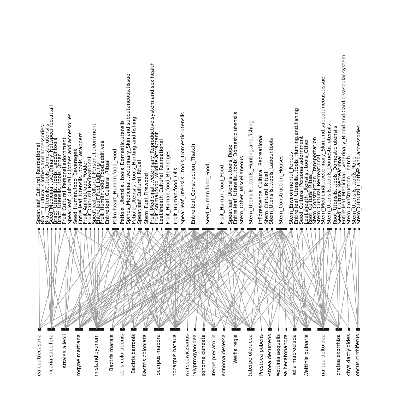
By now, you are familiar using the bipartite and igraph library, so this will be a refresher. Let’s plot one indigenous knowledge network to visualize the two types of nodes and links. First we plot with the bipartite package.
plotweb(Aguacate,col.interaction="grey60",high.lablength=100,
        low.lablength=30,bor.col.interaction="grey60",
        bor.col.high="black",bor.col.low="black",text.rot=90,
        y.width.low=0.01,y.width.high = 0.01,ybig = .1,
        arrow="both.center")
Nodes on one set are plant species (e.g. Attalea allenii),and nodes on the other set are plant services. Each plant service is defined as the concatenation of palm part (e.g. Spear leaf, Stem, Seed, Fruit), use category (e.g., Cultural), and subcategory (e.g. Recreational). There are 10 categories (Animal food, Construction, Cultural, Environmental, Fuel, Human food, Medicinal and veterinary, Toxic, Utensils and tools, and Other uses).
Now we plot with the igraph package.
AG = graph_from_incidence_matrix(Aguacate, weight=T)
polcol = rep("white",dim(Aguacate)[2])# plant services nodes
plantcol = rep("black",dim(Aguacate)[1])# plant species nodes
clrs = rbind(as.matrix(plantcol),as.matrix(polcol))
V(AG)$color = clrs
V(AG)$frame.color = "grey50"
E(AG)$width = E(AG)$weight/1.5
E(AG)$color = "black"
V(AG)$label = ""
plot.igraph(AG, layout=layout.bipartite
            ,vertex.size=5,bg="black",asp = .5,
            edge.width = 1,
            margin=0.1)
11.3 Turnover in plant-service interactions
Now that we are familiar with the data, let’s continue now to assess how biological and cultural heritage jointly influence the structure of indigenous knowledge networks across our study area. One way to do this is by decomposing the turnover in plant–service interactions between indigenous communities. We will use a method that was proposed in the following article: Poisot et al. 2012. To do this we first build a list of networks:
webs <- list(Aguacate, AltoIvon, Angostura, Aviacion, BuenaVista, Camaritagua, CentroProvidencia, Chiguilpe, Correo, Curare, CusuChico, Dureno, ElChino, Illipanayuyo, Irimo, Juisanoy, Kapawi, Kusutkau, LamasWayku, Mayo, Mindo, Motacuzal, Munaypata, Nanegalito, NuevaSamaria, NuevoProgreso, Octubre, Pacuya, PalmaReal, Peripa, Pucasucho, PuertoPervel, PuertoQuito, PuertoYaminahua, Sanandita, SanAntonio, SanBenito, SanIsidro, SanMartin, SanMartinDeAmacayacu, SanSilvestre, SantaAna, SantaMaria, SantaRosa, SantaRosaDeMaravilla, Santiago, SantoDomingoBolivia, Secejsama, Sibundoy, TresArroyos, UnionProgreso, Villanueva, VillaSantiago, Wayusentsa, Yamayakat, Yucuna, Zabalo)Then, taking the list of networks as matrices, we use the prepare_networks function to get a list of igraph objects.
webs_list <- prepare_networks(webs)Don’t worry if you get a Warning message like this one:
Warning message: In name_networks(w): It is recommended to give names to your networks. I've done it for you.
Once we have a list of igraph objects, we can calculate the pairwise beta-diversity components with the network_betadiversity function. This can take a long time to run, so I have already done it for you. To do this you would need to run the following command:
webs_betadiversity <- network_betadiversity(webs_list) The previous function yields the following result.
head(webs_betadiversity)## i j S OS WN ST
## 1 network_1 network_2 0.6142857 0.3888889 0.8650307 0.4761418
## 2 network_1 network_3 0.5465116 0.3255814 0.8402204 0.5146390
## 3 network_1 network_4 0.6307692 0.3714286 0.8461538 0.4747253
## 4 network_1 network_5 0.6470588 0.3846154 0.8406375 0.4560221
## 5 network_1 network_6 0.5686275 0.3392857 0.8422175 0.5029318
## 6 network_1 network_7 0.5555556 0.4285714 0.8656126 0.4370412What do the variables in the columns mean?
- i / j: are the pair of networks being compared.
- S: Dissimilarity in the species composition of communities
- OS: Dissimilarity of interactions established between species common to both communities
- WN: Dissimilarity of interactions
- ST: Dissimilarity of interactions due to species turnover
Using this method allows us to decompose the total dissimilarity between two given indigenous knowledge networks (referred to as “β” in the PNAS paper, or “WN” in the “webs_betadiversity” results calculated above) into two components:
That of plants and services (node) turnover (“βbio” in the PNAS paper, or “ST” in “webs_betadiversity”): where differences in the presence/ absence of links between plants and the services they provide are the result of a plant being present in one community but not in the other.
That of indigenous knowledge (link) turnover (“βcul” or “OS”): where differences in the presence/absence of links between plants that co-occur in both communities and the services they provide are a consequence of the cultural knowledge that one community, but not the other, has on the service that plant provides.
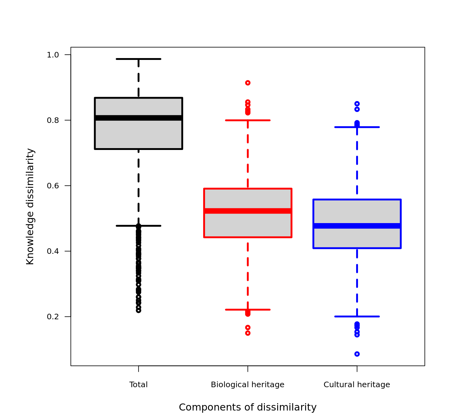
Additionally, by assessing the relative importance of each component we can understand if knowledge networks are shaped by biological heritage (βbio/β or “ST/WN” close to one) or by cultural heritage (βcul/β or “OS/WN” close to one). Let’s calculate the relative importance, and depict this with a boxplot.
par(mfrow=c(1,1),mar=c(4,6,4,4),bg="white")
BiologicalHeritage<-webs_betadiversity$ST/webs_betadiversity$WN
CulturalHeritage<-webs_betadiversity$OS/webs_betadiversity$WN
boxplot(webs_betadiversity$WN,BiologicalHeritage,CulturalHeritage,
        names=c("Total","Biological heritage","Cultural heritage"),
        las=1,outcol=c("black","red","blue"),
        whiskcol=c("black","red","blue"),
        boxcol=c("black","red","blue"),
        medcol=c("black","red","blue"),
        staplecol=c("black","red","blue"),
        outcex=.8,cex.axis=0.8, cex.lab=1,lwd=3,
        pars = list(boxwex = 0.8, staplewex = 0.5, outwex = 0.5),
        xlab="Components of dissimilarity",
        ylab="Knowledge dissimilarity")
11.4 Indigenous knowledge metaweb
So far, we have been comparing pairs of indigenous knowledge networks. In the following section, we will take a macroscopic vision and aggregate the 57 indigenous knowledge networks to build what we refer to as an ‘indigenous knowledge metaweb’. This indigenous knowledge metaweb is simply the global knowledge that communities have of the services provided by all plants occurring in the study area. Getting the distance between a network and its metaweb is easy with the “beta_os_prime” function of the betalink package. This can take a long time to run, so I’ve done it for you. To run the analysis you would enter the following command.
beta_prime<-beta_os_prime(webs_list)There will be 57 β′values, one for each indigenous knowledge network.
length(beta_prime)## [1] 57The higher the β′value, the greater the distance of an indigenous knowledge network to the metaweb (or fewer knowledge).
beta_prime## network_1 network_2 network_3 network_4 network_5 network_6 network_7
## 0.2981818 0.3000000 0.4894895 0.3694915 0.4313725 0.4038877 0.3375661
## network_8 network_9 network_10 network_11 network_12 network_13 network_14
## 0.3119534 0.4615385 0.4345992 0.3497537 0.4798206 0.4023669 0.4702703
## network_15 network_16 network_17 network_18 network_19 network_20 network_21
## 0.3392070 0.3932584 0.4814815 0.4796748 0.3318182 0.4809160 0.3383459
## network_22 network_23 network_24 network_25 network_26 network_27 network_28
## 0.4188034 0.5126050 0.3496933 0.3684211 0.5703704 0.3851852 0.5268293
## network_29 network_30 network_31 network_32 network_33 network_34 network_35
## 0.2946058 0.3472803 0.4285714 0.2683897 0.4181818 0.4621849 0.4947368
## network_36 network_37 network_38 network_39 network_40 network_41 network_42
## 0.4263566 0.3882353 0.4566474 0.4614221 0.3424947 0.4507772 0.4903475
## network_43 network_44 network_45 network_46 network_47 network_48 network_49
## 0.3842482 0.4204545 0.4534884 0.4077670 0.3836478 0.4336283 0.4159292
## network_50 network_51 network_52 network_53 network_54 network_55 network_56
## 0.4424242 0.4285714 0.3136364 0.3846154 0.4622222 0.3313609 0.4242928
## network_57
## 0.5044248What is the range of variation, mean and standard deviation in communities’ dissimilarity to the metaweb?
range(beta_prime)## [1] 0.2683897 0.5703704mean(beta_prime)## [1] 0.4111903sd(beta_prime)## [1] 0.06680852Looking at the values, we see that there is a twofold range of variability in this amount across communities (range, 0.27–0.57; mean, 0.41 ± 0.07). This indicates there is strong variation between communities in their dissimilarity to the metaweb.
11.5 Keystone communities
Based on to the previous exercise, we know that communities are not alike in the amount of indigenous knowledge they contain. So, by quantifying now how much communities deviate from the metaweb, and linking information on community population size, we can classify communities into the following:
11.5.1 1. Standard communities (within one SD from the mean β′ value)
sd1<-mean(beta_prime)+sd(beta_prime)
sd1inf<-mean(beta_prime)-sd(beta_prime)
standard<-which(beta_prime<sd1&beta_prime>sd1inf)
standard
## network_4 network_5 network_6 network_9 network_10 network_11 network_13
## 4 5 6 9 10 11 13
## network_14 network_16 network_22 network_24 network_25 network_27 network_30
## 14 16 22 24 25 27 30
## network_31 network_33 network_34 network_36 network_37 network_38 network_39
## 31 33 34 36 37 38 39
## network_41 network_43 network_44 network_45 network_46 network_47 network_48
## 41 43 44 45 46 47 48
## network_49 network_50 network_51 network_53 network_54 network_56
## 49 50 51 53 54 5611.5.2 2. Sink communities (βi′> one SD from the mean β′ value)
sink<- which(beta_prime>=sd1)
sink
## network_3 network_12 network_17 network_18 network_20 network_23 network_26
## 3 12 17 18 20 23 26
## network_28 network_35 network_42 network_57
## 28 35 42 5711.5.3 3. Source communities (βi′< one SD from the mean β′ value and a human population size >= 1,000)
source_com <- which(beta_prime<=sd1inf)
source_com
## network_1 network_2 network_7 network_8 network_15 network_19 network_21
## 1 2 7 8 15 19 21
## network_29 network_32 network_40 network_52 network_55
## 29 32 40 52 55You will see that this code is the same as below for keystones. To differentiate from keystones, we need human population size data (see “community_classification.csv”).
beta_corr<-read.csv("~/ecological_networks_2022/downloads/Data/04-06_socio-ecological_networks/community_classification.csv")
beta_corr$Community_size
## [1] 312 500 180 300 240 60 100 130 260 130 150 450
## [13] 550 150 350 2000 220 80 1200 100 1500 30 80 3200
## [25] 80 NA 180 150 300 130 280 1500 1500 100 60 90
## [37] 90 50 500 430 100 450 250 500 50 5800 220 100
## [49] 13000 128 300 200 120 150 1000 160 170Now that we know the population size, we determine which communities meet the criteria of SD and have a human population size >= 1000.
intersect(which(beta_prime<=sd1inf),which(beta_corr$Community_size >= 1000))## [1] 19 21 32 55The communities are: 19, 21, 32 and 55.
11.5.4 4. Keystone communities (βi′< one SD from the mean β′ value, <= 500 individuals)
keystone<- which(beta_prime<=sd1inf)
keystone
## network_1 network_2 network_7 network_8 network_15 network_19 network_21
## 1 2 7 8 15 19 21
## network_29 network_32 network_40 network_52 network_55
## 29 32 40 52 55Let’s look at the size of population again.
beta_corr$Community_size## [1] 312 500 180 300 240 60 100 130 260 130 150 450
## [13] 550 150 350 2000 220 80 1200 100 1500 30 80 3200
## [25] 80 NA 180 150 300 130 280 1500 1500 100 60 90
## [37] 90 50 500 430 100 450 250 500 50 5800 220 100
## [49] 13000 128 300 200 120 150 1000 160 170To differentiate from “source” communities, here we need to know which communities have <= 500 of human population size (see “community_classification.csv”).
intersect(which(beta_prime<=sd1inf), which(beta_corr$Community_size <= 500))## [1] 1 2 7 8 15 29 40 52They are the following communities: 1, 2, 7, 8, 15, 29, 40 and 52.
In summary, by decomposing the dissimilarity of pairs of indigenous knowledge networks into the turnover of nodes and links, and assessing the relative importance of each component, we can better understand the local structure of indigenous knowledge networks and the importance of biological vs. cultural heritage in explaining knowledge network turnover. Aggregating all local knowledge networks, in turn, allows us to build a metaweb of indigenous knowledge and classify them into e.g. keystone networks on the basis of their proximity to this metaweb and their human population size.
11.6 Correlates of dissimilarity
To end our exercise of socio-ecological networks, we will explore whether differences in the dissimilarity of local communities to the metaweb (β′) are related to:
- the fraction of species in each community,
- the fraction of services in relation to the metaweb.
11.6.1 Fraction of species in each community
For this, let’s read the “community_classification.csv” which contains additional variables:
beta_corr<-read.csv("~/ecological_networks_2022/downloads/Data/04-06_socio-ecological_networks/community_classification.csv")
names(beta_corr)
## [1] "Network" "Network_name" "Country"
## [4] "Ecoregion" "Beta_os" "Potential_species"
## [7] "Non.used_species" "Used_species" "Fraction_all_species"
## [10] "No_informants" "Potential_uses" "Non.used_uses"
## [13] "Used_uses" "Fraction_all_uses" "Type"
## [16] "Lat" "Lon" "Community_size"The variables of interest are “Beta_os” (or β′), “Fraction_all_species” and “Fraction_all_uses” (or fraction of services). First, let’s standardize these variables to a mean of 0 and standard deviation of 1:
betaos<-scale(beta_corr$Beta_os)
species<-scale(beta_corr$Fraction_all_species)
services<-scale(beta_corr$Fraction_all_uses)
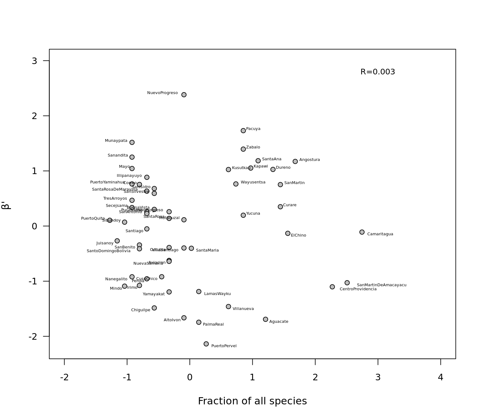
Now let’s run the correlation test between the fraction of all species and β′ and plot the results:
cor.test(species, betaos)##
## Pearson's product-moment correlation
##
## data: species and betaos
## t = 0.024402, df = 55, p-value = 0.9806
## alternative hypothesis: true correlation is not equal to 0
## 95 percent confidence interval:
## -0.2574981 0.2636320
## sample estimates:
## cor
## 0.003290337Finally we plot the correlation, we add correlation value to plot and the community names.
plot.default(species,betaos, pch=21,cex.axis=.9,las=1,ylab=expression(paste(beta,"' "))
     ,xlab="Fraction of all species",bg="grey",xlim=c(-2,4),ylim=c(-2.2,3))

text(3,2.8, "R=0.003",cex=0.8,col="black")

textxy(species,betaos,beta_corr$Network_name,cex=0.4,offset = .7)
11.6.2 Fraction of services in relation to the metaweb
cor.test(services,betaos)##
## Pearson's product-moment correlation
##
## data: services and betaos
## t = -2.6396, df = 55, p-value = 0.01078
## alternative hypothesis: true correlation is not equal to 0
## 95 percent confidence interval:
## -0.54800681 -0.08190962
## sample estimates:
## cor
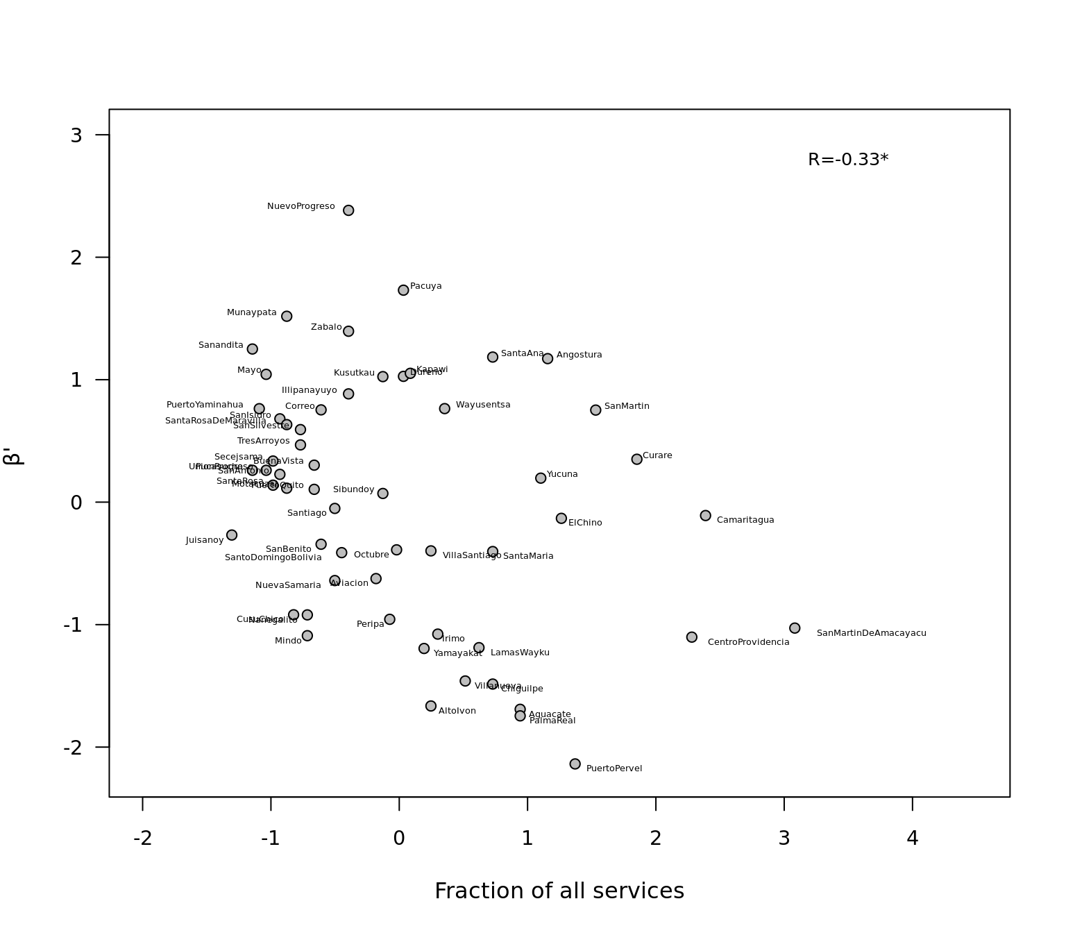
## -0.3353205Finally we plot the correlation, we add correlation value to plot and the community names.
plot.default(services,betaos,pch=21,ylab=expression(paste(beta,"' ")),
     xlab="Fraction of all services",xlim=c(-2,4.5),las=1,cex.axis=.9,bg="grey",ylim=c(-2.2,3))

text(3.5,2.8, "R=-0.33*",cex=0.8,col="black")

textxy(services,betaos,beta_corr$Network_name,cex=0.4,offset = .7)
In summary, we see differences in the dissimilarity of local communities to the metaweb were unrelated to the fraction of species each community contained, but were significantly and negatively related to the fraction of services in relation to the metaweb. Thus, keystone communities are not as defined by their species pool but, rather, by their people’s knowledge. This may be analogous to the species–area relationship of biogeography, whereby as human communities grow in size, their ability to explore nature’s services may increase, fostering more innovations.
11.7 Exercises
- Test and plot the relationship between another variable and β′: for example, what is the relationship between the number of informants and β′? Why do you think this is so?
# Enter your code and text in the file: "AssignmentMailbox/04-06_socio-ecological_networks/S_04-06_socio-ecological_networks.R"- Which indigenous community has more indigenous knowledge when compared to the metaweb? Which has the least?
# Enter your text in the file: "AssignmentMailbox/04-06_socio-ecological_networks/S_04-06_socio-ecological_networks.R"- In the paper we simulated the collapse of the indigenous knowledge metaweb by removing plant species nodes (following the inverse order of plant species’ geographic range) and links (removing the least-cited links first) and then measured how the fraction of removed plant nodes or links affects the mean size of the largest remaining cluster after 1,000 simulations (see pg. 3 in th paper). Considering the unprecedented impacts that humans have on ecosystems, what other criteria besides geographic range would you suggest to rank plant nodes when removing them from the metaweb?
# Enter text in the file: "AssignmentMailbox/04-06_socio-ecological_networks/S_04-06_socio-ecological_networks.R"- In this exercise we have focused on indigenous-knowledge networks. Can you cite two examples of socio-ecological networks? For each of them, what would be the nodes on one set, the nodes on the other set, and the links represent?
# Enter text in the file: "AssignmentMailbox/04-06_socio-ecological_networks/S_04-06_socio-ecological_networks.R"