9 Simulating foraging

Matthew Hutchinson
session 31/03/2022

9.1 What we’re going to do

The aim of today’s session is to predict the structure of food-webs. First, we will ask what foods a specific animal should eat. For this, we will use optimal foraging theory, which gives each potential food a “value” based on its abundance, energy content, and difficulty for the animal to catch and consume. Next, we will scale these ideas up to the level of an entire food-web using the Allometric Diet Breadth Model (ADBM; as proposed by Petchey et al. 2008 PNAS). Finally, we will explore how these expectations change when we alter the available foods and the predator’s ability to catch them.

9.2 1. What is the optimal diet?

To answer this question, we first need to know whose diet we are going to predict. For this exercise, let’s say that we are studying leopards (Panthera pardus) in the Serengeti Ecosystem in Tanzania. The Serengeti is famed for its dense and diverse populations of large herbivores (otherwise known as leopard food). If a Serengeti leopard wants to have the most profitable diet it can (i.e., if it wants to forage in an optimal way), which herbivores should it eat? Let’s figure it out.

First, we need to know the encounter rate between leopards and each potential prey species. To compute that, we can divide the number of individuals are there of each herbivore species by the size of the ecosystem. According to George Schaller’s work there, we have the following herbivore population sizes:

# list the herbivore species present
species <- c('Wildebeest', 'Zebra', 'ThomsonsGazelle', 'GrantsGazelle', 'Eland', 'Topi', 'Hartebeest', 'Impala', 'Waterbuck', 'Giraffe', 'Warthog', 'Buffalo', 'Reedbuck', 'Bushbuck')

# read in the abundance of each herbivore
abund <- c(410000, 140000, 180000, 10000, 7000, 27000, 18000, 65000, 3000, 8000, 15000, 50000, 2500, 2500)
names(abund) <- species

# what is the size of the ecosystem in square kilometers?
serengeti_size <- 30000

# herbivore density is the population size divided by the ecosystem size
density <- abund/serengeti_size

Okay, now we have a measure of each prey species’ availability to hungry leopards. Now we need to estimate how much energy a leopard gets from eating each of the different herbivore species. A good way to estimate this is based on the body mass of each prey species. We can estimate the energy each species represents by converting its weight to calories and then converting calories to joules of energy. In this case, we will use the average adult body mass as reported from Kingdon’s Mammals of Africa books. Let’s read in those values.

# read in the body mass of each herbivore
mass <- c(182.05, 233.45, 18.3, 52.1, 397, 119.5, 134.35, 49.5, 201, 1010.1, 68.05, 598.7, 50, 35) 
names(mass) <- species

# to calculate energy, we first convert mass to grams, then turn that into calories by multiplying it by the number of calories per gram, and convert calories to joules with the number of joules per calorie. Finally, to make the numbers more reasonable we convert the energy estimates from joules to megajoules
mass_in_grams <- mass*1000
energy_in_calories <- mass_in_grams*1093
energy_in_joules <- energy_in_calories*4.184
energy <- energy_in_joules/1000000

The last two values that we need for each species are the trickiest to calculate. The first one is handling time; how long does it take a leopard to pursue, kill, and eat each prey species? The second one is the attack rate; if a leopard encounters a herbivore, what is the chance that it attacks it? To calculate both of these values, we need to (i) know how much our leopard weighs, and (ii) make some assumptions about how leopards choose whether to eat prey larger or smaller than themselves.

# let's use the Kingdon books again to find the weight of a leopard
leo_mass <- 49.75

For handling time, we make the assumption that leopards need more time to catch, kill, and digest larger prey. We can express that idea like this (using the formulation from Petchey et al. 2008 PNAS):

# first we need to choose a value for the parameter b, which helps determines the maximum number of times a prey's weight can be bigger than the leopard's
b = 4
handling <- 1/(b-(mass/leo_mass))

# however when mass/leo_mass is greater than b, we assign handling time to infinite
handling[which(mass/leo_mass >= b)] <- Inf

# to understand how handling time changes with prey and predator body mass, let's plot those changes
# remember with this plot that the x-axis is prey:predator mass so 1 represents when prey and leopards are the same size, <1 means the leopard is bigger than the prey, >1 prey bigger than a leopard
plot(mass/leo_mass, handling)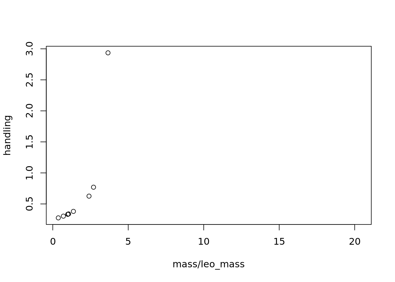

# and the effect of changing the b parameter
alt_b <- 2
alternate_handling <- 1/(alt_b-(mass/leo_mass)) 
alternate_handling[which(mass/leo_mass >= alt_b)] <- Inf
plot(mass/leo_mass, alternate_handling)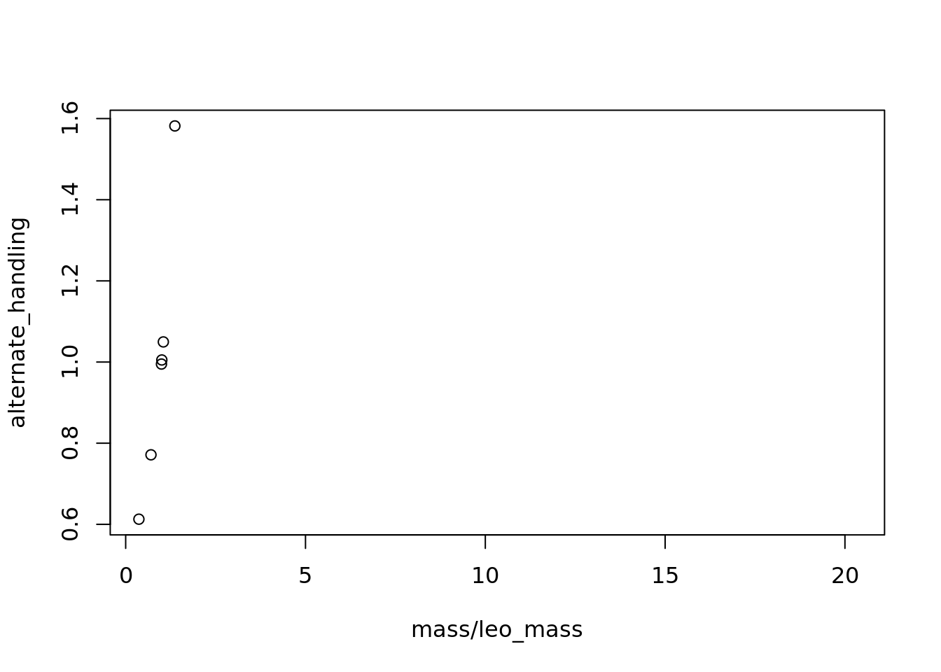

Next, we calculate the attack rate. Again, we will follow the formulation from Petchey et al. here:

# here we also need to choose the values of some parameters to determine the rate at which leopards attack each prey species based on their size
a = 0.001
ai = -0.5
aj = 2
attack <- a*mass^ai*leo_mass^aj

# to understand how attack rate changes with prey and predator body mass, let's plot it
# remember with this plot that the x-axis is prey:predator mass so 1 represents when prey and leopards are the same size, <1 means the leopard is bigger than the prey, >1 prey bigger than a leopard
plot(mass/leo_mass, attack)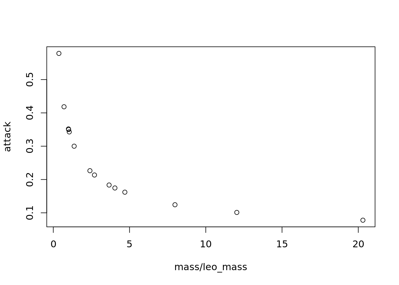

# if we change the ai parameter, how does the relationship change?
alt_ai=-0.001
alt_attack <- a*mass^alt_ai*leo_mass^aj
plot(mass/leo_mass, alt_attack)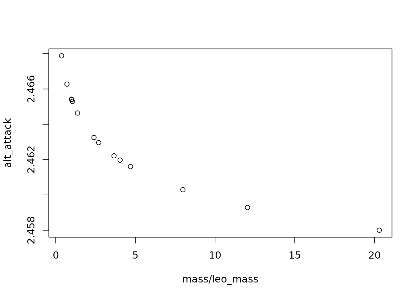

Okay! Now we are ready to compute the optimal diet for Serengeti leopards. To do that, we bring together all of the different values we have calculated.

# first we calculate how much profit the leopard gets from eating a prey species; we divide energy by handling time and sort them from most profitable to least
profit <- energy/handling
profit_sorted <- rev(sort(profit))

# now we introduce a function that will evaluate the profit a leopard gets from eating a certain diet
diet_function <- function(prey, attack, density, energy, handling){
    a_rate <- attack[which(names(attack) %in% prey)]
    dens <- density[which(names(density) %in% prey)] 
    h_time <- handling[which(names(handling) %in% prey)]
    e <- energy[which(names(energy) %in% prey)]
    total_profit <- sum(dens*a_rate*e)/(1+sum(dens*a_rate*h_time)) 
    return(total_profit)
}

# lets see how much energy a leopard gets from each diet
energy_intake <- sapply(1:length(species), function(x) diet_function(prey=names(profit_sorted[1:x]), attack, density, energy, handling))
diet_items <- names(profit_sorted)[1:which(energy_intake == max(energy_intake))]

# okay so let's see which species are in the most profitable diet
print(diet_items)

## [1] "Topi"            "Warthog"         "Hartebeest"      "GrantsGazelle"  
## [5] "Reedbuck"        "Impala"          "Bushbuck"        "ThomsonsGazelle"

# using the rate at which leopards encounter and attack each prey species, we can estimate how much of the leopards diet comes from each prey species
capture_rate <- density*attack
capture_rate <- capture_rate[which(names(capture_rate) %in% diet_items)]

# we then sample 1000 times from this values to estimate how often a leopard eats each of the prey in its optimal diet
diet <- sample(names(capture_rate), 1000, prob=as.numeric(capture_rate), replace=TRUE)
diet <- (table(diet)/1000)*100

print(diet)

## diet
##        Bushbuck   GrantsGazelle      Hartebeest          Impala        Reedbuck 
##             0.7             2.0             2.5            15.4             0.4 
## ThomsonsGazelle            Topi         Warthog 
##            72.4             4.1             2.5

Okay, so in the end, we found that Serengeti leopards are expected to eat eight different prey species and that Thomson’s gazelles (Eudorcas thomsonii) account for >70% of the diet. So, how does this compare to what leopards actually eat in the Serengeti? If we go back to Schaller’s book, we see that nine prey species are found in leopard diets. Six species are in common between the two diets, but we predict that leopards will eat impala (Aepyceros melampus) and bushbuck (Tragelaphus scriptus) and these are not found in the diet whereas the true diet includes wildebeest (Connochaetes taurinus) and plains zebra (Equus quagga) but these are not predicted to be in the diet. When we look at the proportional composition of the diet, Thomson’s gazelles dominate leopard diets (63% of kills) just as we predict (73.4% of diet). However, our model suggests that then next most common prey species should be impala (we predict they are 15.6% of the diet) but the diet records from Schaller indicate no consumption of impala by Serengeti leopards. Instead, the diet records state that reedbuck (Redunca redunca) are the second most important prey item (11.6% of kills); in our model they are just 0.7%. Clearly, our model is capturing some but not all of the factors determining leopard feeding choices in the Serengeti. Why do you think this is? Keep thinking about this, because we will return to it later.

9.3 Predicting the interactions in an entire food-web using optimal-foraging theory

Now that we’ve predicted the diet of one species, why not do the same for an entire food-web? We’ll use the same set of steps as for leopard diets, but let’s imagine this food-web is from a Fijian coral reef. The reason for this change is that we can’t predict the Serengeti food-web just using the Allometric Diet Breath Model and body mass (because otherwise it would predict elephants to eat lions!)

First, let’s generate the same parameter set that we used for leopard diets.

library(igraph)

set.seed(2022)

species <- 50
species_names <- c(letters[1:25], LETTERS[1:25])

# we'll create a log-normally distributed set of body masses for our fish community because this pattern is commonly observed in ecological communities
mean_log_mass <- 1
sd_log_mass <- 0.2 
mass <- exp(rlnorm(species, mean_log_mass, sd_log_mass))
names(mass) <- species_names

# density/abundance tends to be related to non-linearly to body mass (see Damuth 1981 "Population density and body size in mammals")
density_scaling <- -0.75
density <- exp(density_scaling*log(mass) + 4.23)
names(density) <- species_names

# as before, we can estimate energy available to a predator based on each species' body mass
mass_in_grams <- mass*1000
energy_in_calories <- mass_in_grams*1093
energy_in_joules <- energy_in_calories*4.184
energy <- energy_in_joules/1000000
names(energy) <- species_names

You’ll notice that we have computed handling time or attack rates yet. Because handling time and attack rate depends on the size of the predator as well as the prey, we need to calculate these separately for each species, so we will do that at the next step.

# To estimate the food-web structure, we will first estimate the diet of each species and then join those together into a food-web
# to that, we will use the same function from earlier, but this time make it run once for each species (i.e., when each species is a predator)

diets <- list() # this creates an place to save our results
for(i in 1:length(species_names)){
    
    predator <- species_names[i]
    print(predator) # print out which species our is
    predator_mass <- mass[which(names(mass) == predator)]
    prey_mass <- mass[-which(names(mass) == predator)]
    prey_energy <- energy[-which(names(energy) == predator)]
    prey_density <- density[-which(names(density) == predator)]
    prey <- species-1

    # let's calculate the handling time and attack rate that for all the species when species i is the predator
    b = 1
    handling <- 1/(b-(prey_mass/predator_mass))
    handling[which(prey_mass/predator_mass >= b)] <- Inf
    
    a = 0.001
    ai = -0.5
    aj = 2
    attack <- a*prey_mass^ai*predator_mass^aj

    # now let's compute the optimal diet
    profit <- prey_energy/handling
    profit_sorted <- rev(sort(profit))
    energy_intake <- sapply(1:prey, function(x) diet_function(prey=names(profit_sorted[1:x]), attack, prey_density, prey_energy, handling))

    # finally let's save the predator's optimal diet
    diets[[i]] <- names(profit_sorted)[1:which(energy_intake == max(energy_intake))]
    names(diets)[i] <- predator
}

## [1] "a"
## [1] "b"
## [1] "c"
## [1] "d"
## [1] "e"
## [1] "f"
## [1] "g"
## [1] "h"
## [1] "i"
## [1] "j"
## [1] "k"
## [1] "l"
## [1] "m"
## [1] "n"
## [1] "o"
## [1] "p"
## [1] "q"
## [1] "r"
## [1] "s"
## [1] "t"
## [1] "u"
## [1] "v"
## [1] "w"
## [1] "x"
## [1] "y"
## [1] "A"
## [1] "B"
## [1] "C"
## [1] "D"
## [1] "E"
## [1] "F"
## [1] "G"
## [1] "H"
## [1] "I"
## [1] "J"
## [1] "K"
## [1] "L"
## [1] "M"
## [1] "N"
## [1] "O"
## [1] "P"
## [1] "Q"
## [1] "R"
## [1] "S"
## [1] "T"
## [1] "U"
## [1] "V"
## [1] "W"
## [1] "X"
## [1] "Y"

Now we have predicted the diet for every species in the food-web. Now let’s make and explore our food-web!

# first of all let's make our food-web

foodweb <- matrix(0, nrow=species, ncol=species)
colnames(foodweb) <- species_names
rownames(foodweb) <- species_names

# let's take a look at what we have so far
head(foodweb)

##   a b c d e f g h i j k l m n o p q r s t u v w x y A B C D E F G H I J K L M N
## a 0 0 0 0 0 0 0 0 0 0 0 0 0 0 0 0 0 0 0 0 0 0 0 0 0 0 0 0 0 0 0 0 0 0 0 0 0 0 0
## b 0 0 0 0 0 0 0 0 0 0 0 0 0 0 0 0 0 0 0 0 0 0 0 0 0 0 0 0 0 0 0 0 0 0 0 0 0 0 0
## c 0 0 0 0 0 0 0 0 0 0 0 0 0 0 0 0 0 0 0 0 0 0 0 0 0 0 0 0 0 0 0 0 0 0 0 0 0 0 0
## d 0 0 0 0 0 0 0 0 0 0 0 0 0 0 0 0 0 0 0 0 0 0 0 0 0 0 0 0 0 0 0 0 0 0 0 0 0 0 0
## e 0 0 0 0 0 0 0 0 0 0 0 0 0 0 0 0 0 0 0 0 0 0 0 0 0 0 0 0 0 0 0 0 0 0 0 0 0 0 0
## f 0 0 0 0 0 0 0 0 0 0 0 0 0 0 0 0 0 0 0 0 0 0 0 0 0 0 0 0 0 0 0 0 0 0 0 0 0 0 0
##   O P Q R S T U V W X Y
## a 0 0 0 0 0 0 0 0 0 0 0
## b 0 0 0 0 0 0 0 0 0 0 0
## c 0 0 0 0 0 0 0 0 0 0 0
## d 0 0 0 0 0 0 0 0 0 0 0
## e 0 0 0 0 0 0 0 0 0 0 0
## f 0 0 0 0 0 0 0 0 0 0 0

# so we have a matrix with species' names in the rows and columns and all entries as zero. Now let's fill this with the diets. In this case, and with food-webs more generally, each column represents a species when it is a predator (and each row represents a species when it is prey). To fill the food-web, we will again use a for-loop to run the code for each species

for(i in 1:length(diets)){
    diet <- diets[[i]]
    foodweb[which(rownames(foodweb) %in% diet), which(colnames(foodweb) == names(diets)[i])] <- 1
}

# let's tak another look
head(foodweb) # viola!

##   a b c d e f g h i j k l m n o p q r s t u v w x y A B C D E F G H I J K L M N
## a 0 0 0 0 0 0 0 0 0 0 0 0 0 0 0 0 0 0 0 0 0 0 0 0 0 0 0 0 0 0 0 0 0 0 0 0 0 0 0
## b 0 0 0 0 1 0 0 1 0 1 0 1 0 1 1 1 0 0 0 0 1 1 0 0 1 0 0 1 0 1 1 0 0 1 0 0 0 1 1
## c 0 0 0 0 0 0 0 1 1 1 0 0 0 1 0 0 0 0 0 0 1 1 0 0 0 0 1 1 0 0 1 0 0 0 0 0 0 1 1
## d 0 0 0 0 1 0 0 1 0 1 0 1 0 1 1 1 1 0 0 0 1 1 0 0 1 0 0 1 1 1 1 0 0 1 1 0 0 1 1
## e 1 0 0 0 0 0 0 0 1 0 1 0 0 0 0 0 0 0 1 1 0 0 1 0 0 0 1 0 0 0 0 1 0 0 0 1 1 0 0
## f 0 1 1 1 1 0 1 0 0 0 0 0 1 0 0 0 1 1 0 0 0 0 0 0 1 1 0 0 1 1 0 0 1 1 1 0 0 0 0
##   O P Q R S T U V W X Y
## a 0 0 0 0 0 0 0 0 0 0 0
## b 1 1 0 0 0 1 0 1 1 0 1
## c 0 0 0 0 0 0 0 1 0 0 1
## d 1 1 0 0 0 1 1 1 1 0 1
## e 0 0 1 0 0 0 0 0 0 0 0
## f 0 1 0 1 1 0 1 0 1 1 0

# okay but now we want to know about the structure of our food-web
    # first we can summarize the number of prey per predator species
mean(colSums(foodweb))

## [1] 8.06

    # next let's turn the food-web matrix into a food-web network for R and then measure the connectance or edge density of the network
foodweb_net <- graph_from_adjacency_matrix(foodweb)
edge_density(foodweb_net)

## [1] 0.1644898

    # finally let's plot the network
plot(foodweb_net, edge.arrow.size=0.4, layout=layout_on_sphere)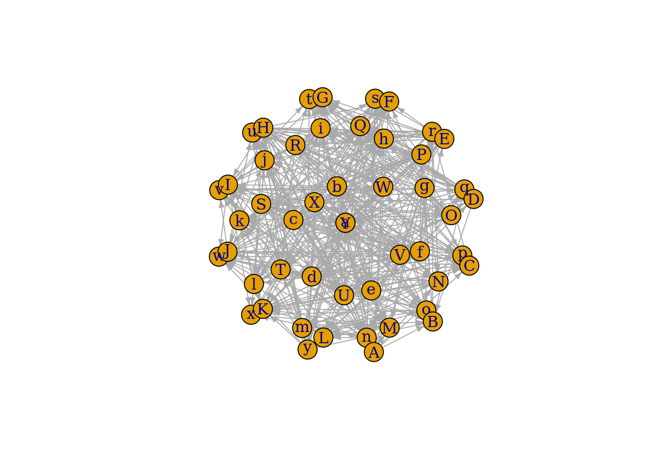

Pretty cool! We started this exercise by choosing a number of species, making an assumption about their body masses, and some assumptions about how body mass determines foraging variables, and we end it with a food-web. The next steps would be to take a real food-web and see how well these assumptions create food-webs that predict the real interactions, but we will leave that for another day.

9.4 Exercises

Send your answers as an email to matthewcraig.hutchinson@uzh.ch

9.4.0.1 Part 1

Return to the first exercise where we predicted leopard diets. In one sentence each, answer the following questions:

What is one biological reason that you can think of why leopards in the Serengeti do not each impala even though our model predicts they should?
How could you change our model so that it also predicts leopards to eat zebra and wildebeest as they do in the Serengeti?
If you could make a more complex model of leopard foraging, what is one additional aspect of hunting behavior or one additional trait of the prey that you could try to include in the model to improve the predictions? How do you think it would help improve the predictions?

9.4.0.2 Part 2

A venture captialist has decided that the Serengeti would be more attractive to tourists if alpine ibex (Capra ibex) are introduced to the ecosystem. They plan to introduce 20000 individuals. You need to evaluate whether or not leopards will eat these ibex and how much of the leopards’ diet they will likely comprise. Compute the optimal leopard diet and estimate how much each species contributes to it using the same approach we used for leopards’ regular diets. In your answer to the question, report the optimal diet after ibex have been introduced and describe how it differs from the leopard’s regular diet (as computed above).

Below are the species list, body masses, and abundances with ibex added.

species <- c('Wildebeest', 'Zebra', 'ThomsonsGazelle', 'GrantsGazelle', 'Eland', 'Topi', 'Hartebeest',
    'Impala', 'Waterbuck', 'Giraffe', 'Warthog', 'Buffalo', 'Reedbuck', 'Bushbuck', 'Ibex')

abund <- c(410000, 140000, 180000, 10000, 7000, 27000, 18000, 65000, 3000, 8000, 15000, 50000, 2500, 2500, 20000)
names(abund) <- species

mass <- c(182.05, 233.45, 18.3, 52.1, 397, 119.5, 134.35, 49.5, 201, 1010.1, 68.05, 598.7, 50, 35, 58.25) 
names(mass) <- species

9.4.0.3 Part 3

Handling time is a notoriously difficult parameter to measure and estimate for feeding interactions. The parameter ‘b’ in the handling-time calculation marks the number of times larger a prey can be for the predator to still, possibly, eat it. Let’s assess the effect it has on our predicted food-web. Repeat the code that we used to make the food-web three times. For the first, change the parameter ‘b’ to 0.5, for the second change it to 1.5, the third to 3. For each new food-web that you create, compute the mean number of prey per predator species and the edge density again. Report these values for each value of b (including when b=1, which is the example value) and describe how the edge density and mean number of prey per predator changes as the parameter ‘b’ increases.