8 Comparing networks in space
Klementyna Gawecka
session 30/03/2022
Slides for this exercise session are available here.
8.1 Introduction
In ecology, we explore how similar two communities are through the concept of beta diversity (β-diversity). Beta diversity is the species turnover between two different communities. This metric refers to how similar or how stable the communities are through space or time. Traditionally, community ecologists have analysed spatial and temporal differences only in species composition, without considering the changes in species interactions or species roles within assemblages (Poisot et al., 2012).
Quantifying to what extent interaction realization varies, both between sites (or across time), and when compared to the metaweb, can help us understand environmental and human impacts on network structure.
The recent applications for quantifying interaction β-diversity support the growing realization that links in a network are not merely contingent on two species co-occurring but are influenced by a series of other factors, which vary over space and time, and that can promote a rearrangement (rewiring) of the interactions (Poisot et al., 2012).
Through the following exercise session, we will learn how to analyse and interpret the interaction β-diversity and how to relate it to the differences in the environmental conditions of the communities.
- Poisot T., Canard D.M., Mouquet, N., Gravel D.: The dissimilarity of species interaction networks. Ecology Letters, 1353-1361 (2012). DOI 10.1111/ele.12002
8.2 Interaction β-diversity
Poisot et al. (2012) proposed that differences in interactions between networks originate from differences in species composition, and because the same species may interact differently in two different communities. Therefore, the interaction β-diversity can be partitioned as:
\[β_{WN} = β_{ST} + β_{OS}\]
Where \(β_{WN}\) is the total dissimilarity of interactions between networks that results from:
\(β_{ST}\): the dissimilarity of interactions due to differences in species composition (species turnover), and
\(β_{OS}\), the dissimilarity of interactions due to rearrangement of interactions (rewiring)
To calculate \(β_{WN}\) and \(β_{OS}\), we will adopt the Whittaker’s dissimilarity measure \(β_{W}\):
\[β_{W}=\frac{a+b+c}{(2a+b+c)/2} - 1\]
Where: \(a\) is the number of interactions that are shared between two networks, \(b\) is the number of interactions that are unique to network 1, and \(c\) is the number of interactions that are unique to network 2.
Note that, while other dissimilarity measures exist, Whittaker’s is widely used in ecology.
Because differences in network structure can arise either through changes in species compositions or realized interactions, there is no obvious analytical solution for \(β_{ST}\). It is calculated as the difference between \(β_{WN}\) and \(β_{OS}\).
8.3 β-diversity in R: example
To calculate we β-diversity in R, will use the package betalink (Poisot, 2016), and the functions betalink and network_betadiversity.
Let’s load the dataset containing networks from the Argentinian ‘sierras’ (Sabatino et al., 2010).
# load network data
sierras_networks <- read.csv('~/ecological_networks_2022/downloads/Data/03-30_comparing_networks_in_space/sierras_networks.csv')

head(sierras_networks)
## site area latitude longitude plant
## 1 Amarante 190 -37.84201 -58.35857 Achyrocline satureoides
## 2 Amarante 190 -37.84201 -58.35857 Achyrocline satureoides
## 3 Amarante 190 -37.84201 -58.35857 Achyrocline satureoides
## 4 Amarante 190 -37.84201 -58.35857 Achyrocline satureoides
## 5 Amarante 190 -37.84201 -58.35857 Achyrocline satureoides
## 6 Amarante 190 -37.84201 -58.35857 Achyrocline satureoides
## pollinator interaction
## 1 Anthomyiidae 1
## 2 Apis mellifera 1
## 3 Augochlorella ephyra 1
## 4 Camponotus sp 1
## 5 Chilicola sp 1
## 6 Mischocyttarus drewseni 1# site names
unique(sierras_networks$site)## [1] "Amarante" "Cinco_Cerros" "Difuntito" "Difuntos" "El_Morro"
## [6] "La_Barrosa" "La_Brava" "La_Chata" "La_Paja" "Piedra_Alta"
## [11] "Vigilancia" "Volcan"
First, we need to transform the data in the data frame into into incidence matrices (with plants as rows and pollinators as columns). We can transform the data simultaneously for all networks and store the matrices in a list. Note that we need packages plyr and reshape2 for this.
library(plyr)
library(reshape2)

nets <- dlply(sierras_networks, .(site), acast, plant~pollinator, sum, value.var="interaction")
You can access the incidence matrix for network Amarante (for example) with nets[[1]] or nets$Amarante.
Finally, we need to transform the interaction matrices into igraph objects using function prepare_networks from betalink package. This is important as the function we will use to calculate the interaction β-diversity works with igraph objects.
library(betalink)

networks <- prepare_networks(nets, directed = FALSE)
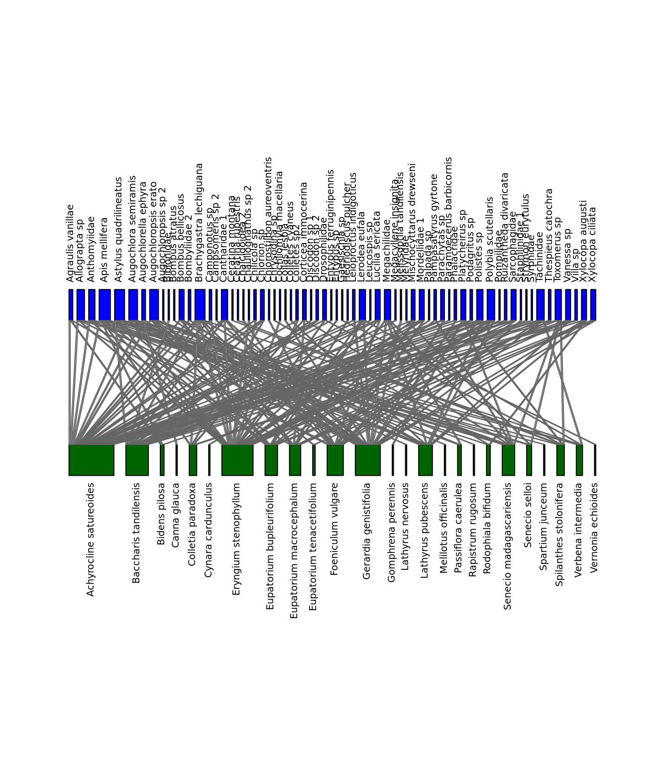
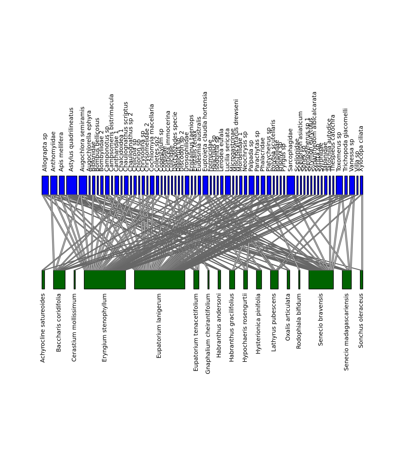
We can visualize the differences between the networks. Let’s look at Difuntos and El_Morro. Note that we need package bipartite for this.
library(bipartite)

plotweb(nets$Difuntos, method="normal", text.rot=90,  bor.col.interaction="gray40",
                plot.axes=F,col.high="blue",labsize = 1, col.low="darkgreen",y.lim=c(-1,3),
                low.lablength=40, high.lablength=40)

plotweb(nets$El_Morro, method="normal", text.rot=90,  bor.col.interaction="gray40",
                plot.axes=F,col.high="blue", col.low="darkgreen",y.lim=c(-1,3),
                low.lablength=40, high.lablength=40)
 Networks of interactions: Difuntos (left) and El_Morro (right). Green represents plants and blue represents pollinators.
network_betaplot(networks$Difuntos, networks$El_Morro,
                 vertex.size=10, vertex.label=NA, directed=FALSE)
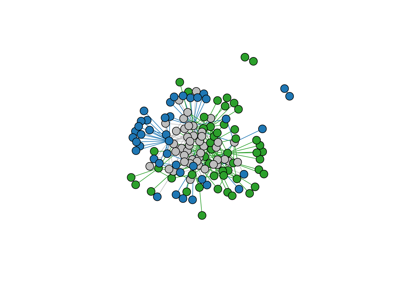
Metaweb highlighting the difference between the two networks. Green represents species present only in Difuntos. Blue represents species present only in El_Morro. Gray represents species present in both sites.
Now, let’s calculate β-diversity between Difuntos and El_Morro using function betalink.
betalink(networks$Difuntos, networks$El_Morro) ## $S
## [1] 0.505618
##
## $OS
## [1] 0.46
##
## $WN
## [1] 0.8363636
##
## $ST
## [1] 0.3763636
We can also calculate β-diversity between all pairs of networks using function network_betadiversity.
betadiversity <- network_betadiversity(networks)

betadiversity
## i j S OS WN ST
## 1 Amarante Cinco_Cerros 0.3564356 0.4934498 0.6768802 0.1834304
## 2 Amarante Difuntito 0.3721973 0.6390977 0.7762238 0.1371260
## 3 Amarante Difuntos 0.4200000 0.5526316 0.8210526 0.2684211
## 4 Amarante El_Morro 0.4421053 0.5244755 0.7914110 0.2669355
## 5 Amarante La_Barrosa 0.3500000 0.5475113 0.7245179 0.1770066
## 6 Amarante La_Brava 0.3936170 0.5023474 0.7047354 0.2023880
## 7 Amarante La_Chata 0.3500000 0.5283843 0.7150396 0.1866553
## 8 Amarante La_Paja 0.3516484 0.4881517 0.6625000 0.1743483
## 9 Amarante Piedra_Alta 0.4123711 0.6864865 0.8370787 0.1505922
## 10 Amarante Vigilancia 0.4205607 0.4470046 0.7215777 0.2745731
## 11 Amarante Volcan 0.3461538 0.4330709 0.6538462 0.2207753
## 12 Cinco_Cerros Difuntito 0.3896714 0.6000000 0.7815534 0.1815534
## 13 Cinco_Cerros Difuntos 0.4315789 0.5882353 0.8071625 0.2189272
## 14 Cinco_Cerros El_Morro 0.4555556 0.4876033 0.7993528 0.3117494
## 15 Cinco_Cerros La_Barrosa 0.4105263 0.5247525 0.7225434 0.1977909
## 16 Cinco_Cerros La_Brava 0.3932584 0.5026455 0.7251462 0.2225007
## 17 Cinco_Cerros La_Chata 0.4000000 0.5098039 0.7237569 0.2139530
## 18 Cinco_Cerros La_Paja 0.3720930 0.5000000 0.7029703 0.2029703
## 19 Cinco_Cerros Piedra_Alta 0.4673913 0.5968992 0.8466077 0.2497084
## 20 Cinco_Cerros Vigilancia 0.4215686 0.5390947 0.7294686 0.1903739
## 21 Cinco_Cerros Volcan 0.3838384 0.4771784 0.6842105 0.2070321
## 22 Difuntito Difuntos 0.4597156 0.7122302 0.9076212 0.1953910
## 23 Difuntito El_Morro 0.4427861 0.4968553 0.7889182 0.2920629
## 24 Difuntito La_Barrosa 0.4786730 0.7172775 0.8701923 0.1529148
## 25 Difuntito La_Brava 0.4673367 0.5833333 0.8300971 0.2467638
## 26 Difuntito La_Chata 0.4502370 0.6701031 0.8518519 0.1817488
## 27 Difuntito La_Paja 0.4093264 0.6062176 0.7962466 0.1900290
## 28 Difuntito Piedra_Alta 0.3756098 0.6100000 0.8092910 0.1992910
## 29 Difuntito Vigilancia 0.4577778 0.6082474 0.8429752 0.2347278
## 30 Difuntito Volcan 0.4703196 0.5392670 0.8123667 0.2730997
## 31 Difuntos El_Morro 0.5056180 0.4600000 0.8363636 0.3763636
## 32 Difuntos La_Barrosa 0.4042553 0.4345550 0.7057221 0.2711671
## 33 Difuntos La_Brava 0.3863636 0.4489796 0.7024793 0.2534997
## 34 Difuntos La_Chata 0.4255319 0.4427861 0.7075718 0.2647857
## 35 Difuntos La_Paja 0.4705882 0.5474453 0.8086420 0.2611967
## 36 Difuntos Piedra_Alta 0.4615385 0.6724138 0.8944444 0.2220307
## 37 Difuntos Vigilancia 0.4158416 0.4666667 0.7241379 0.2574713
## 38 Difuntos Volcan 0.3877551 0.4628099 0.6904762 0.2276663
## 39 El_Morro La_Barrosa 0.4494382 0.5319149 0.7891374 0.2572225
## 40 El_Morro La_Brava 0.4939759 0.4375000 0.8252427 0.3877427
## 41 El_Morro La_Chata 0.4494382 0.5338346 0.8115502 0.2777156
## 42 El_Morro La_Paja 0.3875000 0.4421769 0.6962963 0.2541194
## 43 El_Morro Piedra_Alta 0.4651163 0.5208333 0.8496732 0.3288399
## 44 El_Morro Vigilancia 0.4687500 0.5460993 0.8320210 0.2859217
## 45 El_Morro Volcan 0.4623656 0.4385965 0.8251366 0.3865401
## 46 La_Barrosa La_Brava 0.3522727 0.4732143 0.6589595 0.1857453
## 47 La_Barrosa La_Chata 0.2978723 0.5489362 0.7103825 0.1614463
## 48 La_Barrosa La_Paja 0.4235294 0.5661376 0.7328990 0.1667615
## 49 La_Barrosa Piedra_Alta 0.5164835 0.6423841 0.8425656 0.2001815
## 50 La_Barrosa Vigilancia 0.4059406 0.4732143 0.7177033 0.2444891
## 51 La_Barrosa Volcan 0.4081633 0.4400000 0.6873449 0.2473449
## 52 La_Brava La_Chata 0.3181818 0.5146444 0.6795580 0.1649137
## 53 La_Brava La_Paja 0.4303797 0.4520548 0.7359736 0.2839188
## 54 La_Brava Piedra_Alta 0.4941176 0.6571429 0.8938053 0.2366625
## 55 La_Brava Vigilancia 0.3684211 0.5325670 0.7053140 0.1727470
## 56 La_Brava Volcan 0.3152174 0.4000000 0.5639098 0.1639098
## 57 La_Chata La_Paja 0.4235294 0.4424242 0.7151703 0.2727460
## 58 La_Chata Piedra_Alta 0.4615385 0.5944056 0.8384401 0.2440345
## 59 La_Chata Vigilancia 0.3564356 0.4981818 0.6820276 0.1838458
## 60 La_Chata Volcan 0.3469388 0.5248227 0.6801909 0.1553682
## 61 La_Paja Piedra_Alta 0.4756098 0.5462185 0.8200000 0.2737815
## 62 La_Paja Vigilancia 0.4782609 0.4319527 0.7440000 0.3120473
## 63 La_Paja Volcan 0.4157303 0.4772727 0.7444444 0.2671717
## 64 Piedra_Alta Vigilancia 0.4897959 0.6621622 0.8783455 0.2161833
## 65 Piedra_Alta Volcan 0.4842105 0.7226277 0.9040404 0.1814127
## 66 Vigilancia Volcan 0.3714286 0.4468085 0.6135881 0.1667796
The relative influence of the two components of the total dissimilarity (i.e. \(β_{ST}\) and \(β_{OS}\)) can be expressed in a more intuitive way as fractions \(β_{ST}/β_{WN}\) and \(β_{OS}/β_{WN}\).
library(dplyr)

betadiversity <- betadiversity %>%
  mutate(relative_OS = OS/WN, relative_ST = ST/WN)

head(betadiversity)
## i j S OS WN ST relative_OS
## 1 Amarante Cinco_Cerros 0.3564356 0.4934498 0.6768802 0.1834304 0.7290061
## 2 Amarante Difuntito 0.3721973 0.6390977 0.7762238 0.1371260 0.8233421
## 3 Amarante Difuntos 0.4200000 0.5526316 0.8210526 0.2684211 0.6730769
## 4 Amarante El_Morro 0.4421053 0.5244755 0.7914110 0.2669355 0.6627094
## 5 Amarante La_Barrosa 0.3500000 0.5475113 0.7245179 0.1770066 0.7556905
## 6 Amarante La_Brava 0.3936170 0.5023474 0.7047354 0.2023880 0.7128171
## relative_ST
## 1 0.2709939
## 2 0.1766579
## 3 0.3269231
## 4 0.3372906
## 5 0.2443095
## 6 0.2871829
Finally, let’s calculate the interaction β-diversity between the networks and the metaweb.
A metaweb is the regional pool of species and their potential interactions. A local network is a realization from a regional metaweb.
Understanding the interaction β-diversity between local networks and the metaweb allows us to characterize the diversity of interactions in space, which is the first step in developing a predictive theory of spatial network ecology.
We need to create the metaweb using the function metaweb and join the metaweb with the rest of the networks.
M <- metaweb(networks)
networks$metaweb <- M

print(names(networks))
## [1] "Amarante" "Cinco_Cerros" "Difuntito" "Difuntos" "El_Morro"
## [6] "La_Barrosa" "La_Brava" "La_Chata" "La_Paja" "Piedra_Alta"
## [11] "Vigilancia" "Volcan" "metaweb"Now, in the network object, we have the local networks and the metaweb. β-diversity can now be recalculated using the function network_betadiversity, just like we did it for all the sites.
8.4 Interpertation of R output
S - dissimilarity in species composition \(β_{S}\)
- \(β_{S}=0\): all species co-occur in both networks
- \(β_{S}=1\): no common species in two networks
OS - dissimilarity due to rewiring \(β_{OS}\)
- \(β_{OS}=0\): all links between species that co-occur in the two networks found in the two networks
- \(β_{OS}=1\): no common links between species that co-occur in the two networks found in the two networks
WN - dissimilarity of interactions \(β_{WN}\)
- \(β_{WN}=0\): every link between species found in both networks
- \(β_{WN}=1\): no common links in two networks
ST - dissimilarity due to species turnover \(β_{ST}\)
- \(β_{ST}=0\): no links found between species that occur in one network but not in the other
- \(β_{ST}=1\): every link found in one network not found in the other because the species involved did not co-occur
8.5 Exercises
We have learned how to evaluate the interaction β-diversity on a network dataset. Now, it’s your turn to explore interaction β-diversity among the 12 communities from the Argentinian ‘sierras’, and relate it to the geographical distance between them. Follow these steps:
Step 1
Load the data set called sierras_networks.csv.
Hint: see the example code above
Step 2
Calculate the β-diversity for the 12 communities.
Hint: see the example code above
Step 3
Calculate the geographical distance between the 12 communities using their coordinates, and store it in a dataframe.
Hints:
- Geographical coordinates of sites are provided in
sierras_networks.csv - Use the function
distmfrom packagegeosphere, and the following code to calculate distances between sites
# extract site coordinates
site_coords <- unique(sierras_networks[,c("site","longitude","latitude")])

# create a distance matrix
dist_matrix <- distm(site_coords[,c("longitude","latitude")], fun=distHaversine)
colnames(dist_matrix) = rownames(dist_matrix) = site_coords$site

# transform the distance matrix into a dataframe
network_dist <- dist_matrix %>%
  melt() %>%
  dplyr::rename(i=Var1, j=Var2, distance=value)
Step 4
Join the betadiversity and site distance dataframes.
Hint: use function left_join from dplyr to join the two data frames by columns i and j.
Step 5
Plot the relationship between geographical distance and the different components of interaction β-diversity (\(β_{WN}\), \(β_{ST}/β_{WN}\) and \(β_{OS}/β_{WN}\)).
Hint: you can use the function ggplot (from package ggplot2) with aes(x=distance, y=beta_value, col=beta_component) to colour the plotted data by the three components, but you will need to transform your data frame accordingly.
Questions
Please answer the following questions in your RScripts (use # at the start of each line):
Q1: What is the relationship between geographical distance and interaction β-diversity?
Q2: Is this relationship mainly explained by the species turnover or by the interaction rewiring?
Q3: Throughout this course, you also learned that we can compare the networks using the topology metrics of networks (e.g. nestedness, modularity, connectance). Here, we used interaction β-diversity. What is the difference between using interaction β-diversity and the other metrics? What is the new information that interaction beta diversity offer to us? Explain your answer.
Bonus exercise
Explore the relationship of β-diversity of the sites with the metaweb and the site area.