4 Measuring nestedness
Klementyna Gawecka
session 23/03/2022
Slides for this exercise session are available here.
4.1 Introduction
Nestedness is a measure of the structure of bipartite networks. Ecological networks, such as plant-pollinator networks, are often nested.
There there are many different measures of nestedness. We will focus on a slightly modified version of the NODF measure (Almeida-Neto et al., 2008) which was used, for example, in Fortuna et al. (2019) to investigate networks of bacteria and phages.
The exercises in Part 1 are to be solved on paper. Please take a picture or scan your work, name the file as surname_name followed by the extension (png, jpg, pdf, etc.), and send the file to klementyna.gawecka@uzh.ch.
The exercises in Part 2 must be solved in R and submitted as an RScript.
In the section R Scripts you find code that will help you to solve the exercises in Part 2.
Almeida-Neto, M., Guimarães, P., Guimarães, P.R., Ulrich, W.: A consistent metric for nestedness analysis in ecological systems: reconciling concept and measurement. Oikos, 1227–1239 (2008). DOI 10.1111/j.2008.0030-1299.16644.xh
Fortuna, M.A., Barbour, M.A., Zaman, L., Hall, A.R., Buckling, A. and Bascompte, J.: Coevolutionary dynamics shape the structure of bacteria‐phage infection networks. Evolution 1001-1011 (2019). DOI 10.1111/evo.13731
4.2 R Scripts
The following R function implements the Fortuna et al. (2019) nestedness measure.
compute_nestedness <- function(B){

  # Get number of rows and columns
  nrows <- nrow(B)
  ncols <- ncol(B)

  # Compute nestedness of rows
  nestedness_rows <- 0
  for(i in 1:(nrows-1)){
    for(j in (i+1): nrows){

      c_ij <- sum(B[i,] * B[j,])      # Number of interactions shared by i and j
      k_i <- sum(B[i,])               # Degree of node i
      k_j <- sum(B[j,])               # Degree of node j

      if (k_i == 0 || k_j==0) {next}  # Handle case if a node is disconnected

      o_ij <- c_ij / min(k_i, k_j)    # Overlap between i and j

      nestedness_rows <- nestedness_rows + o_ij
    }
  }

  # Compute nestedness of columns
  nestedness_cols <- 0
  for(i in 1: (ncols-1)){
    for(j in (i+1): ncols){

      c_ij <- sum(B[,i] * B[,j])      # Number of interactions shared by i and j
      k_i <- sum(B[,i])               # Degree of node i
      k_j <- sum(B[,j])               # Degree of node j
      if (k_i == 0 || k_j==0) {next}  # Handle case if a node is disconnected.

      o_ij <- c_ij / min(k_i, k_j)    # Overlap between i and j

      nestedness_cols <- nestedness_cols + o_ij
    }
  }

  # Compute nestedness of the network
  nestedness <- (nestedness_rows + nestedness_cols) / ((nrows * (nrows - 1) / 2) + (ncols * (ncols - 1) / 2))

  return(nestedness)
}
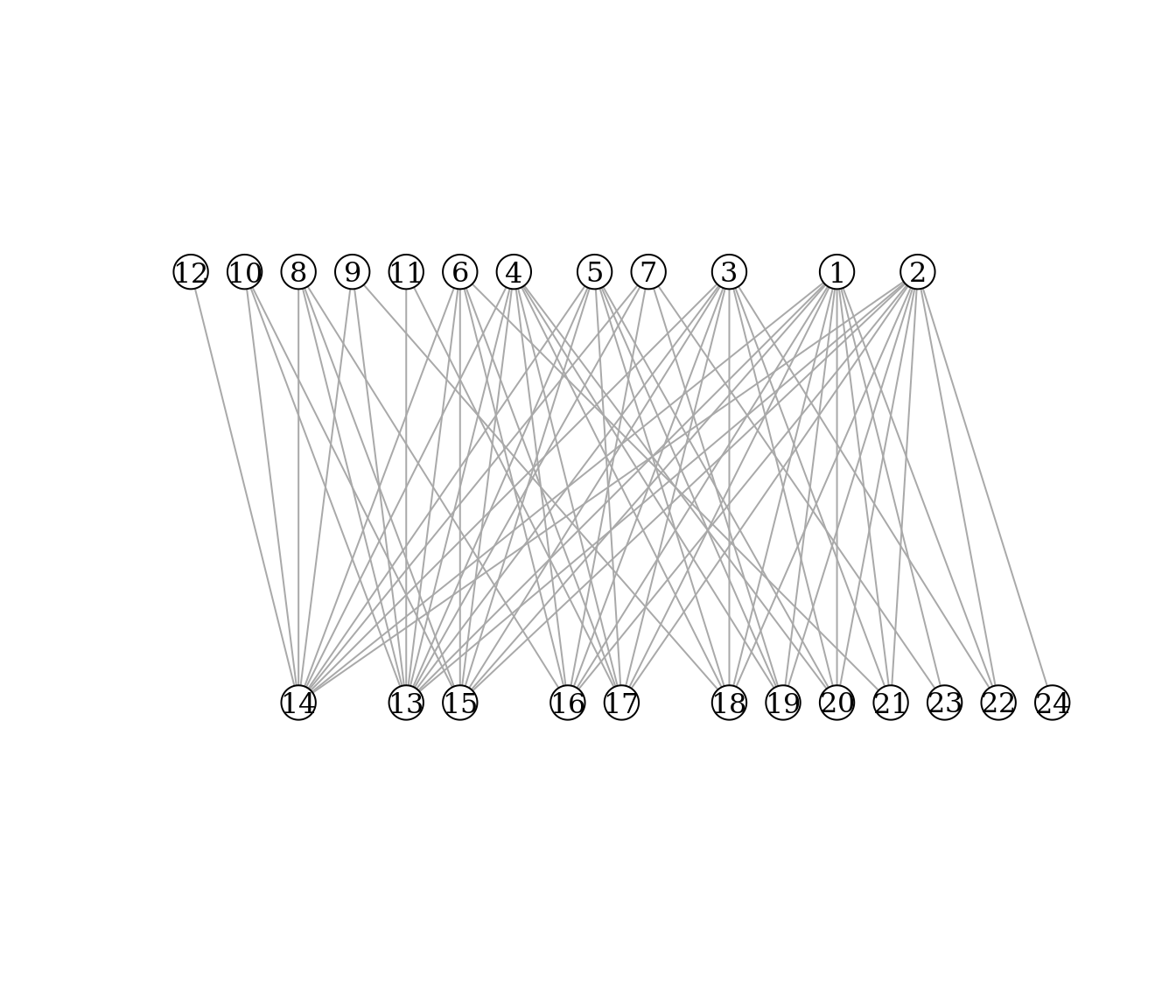
The following code loads a network and plots it using functions from the R igraph package.
The incidence matrix file of the network is available in the code as the object B_example.
# Import the igraph library
library(igraph)

# Convert data into a matrix
B <- as.matrix(B_example)

# Create a bipartite igraph from an incidence matrix
graph <- graph.incidence(B)

# Plot network using bipartite layout
plot(graph,
     layout=layout_as_bipartite,
     vertex.size=8,
     vertex.label.color='black',
     vertex.color='white',
     margin=0.0,
     asp=0.5)
The following code computes the nestedness of the network using the compute_nestedness function defined above.
# Convert data to matrix
B <- as.matrix(B_example)

# Compute network nestedness
compute_nestedness(B)
## [1] 0.88158624.3 Exercises - Part 1 (on paper)
Once you have completed the following exercises on paper, please take a picture or scan your work and name the file as: surname_name followed by the extension (png, jpg, pdf, etc.). Send the file to klementyna.gawecka@uzh.ch.
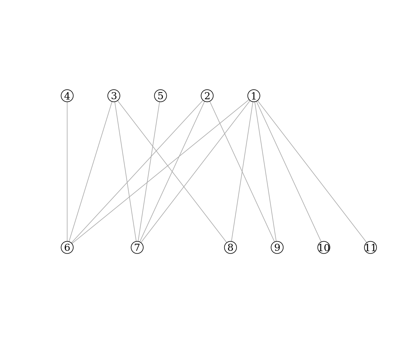
Exercise 1: For the bipartite graph drawn below:
- compute the connectance C
- write down the incidence matrix B

Exercise 2: Compute the nestedness of the bipartite graph defined by the incidence matrix \(B_2\).
\[ \\B_2 = \begin{bmatrix} 1 & 1 & 1 & 1 & 1 & 1 \\ 1 & 1 & 0 & 1 & 0 & 0 \\ 1 & 1 & 1 & 0 & 0 & 0 \\ 1 & 0 & 0 & 0 & 0 & 0 \\ 0 & 1 & 0 & 0 & 0 & 0 \\ \end{bmatrix} \]
4.4 Exercises - Part 2 (R)
Exercise 3: Use R to check the result you obtained in Exercise 2.
Hint: Copy and paste into your Rscript the compute_nestedness function provided in section R Scripts. Use the following code to create the incidence matrix \(B_2\). Then, calculate its nestedness using the compute_nestedness function (see example above).
B2 <- matrix(c(1,1,1,1,0,
               1,1,1,0,1,
               1,0,1,0,0,
               1,1,0,0,0,
               1,0,0,0,0,
               1,0,0,0,0), nrow=5, ncol=6)
Exercise 4: For the mutualistic plant-pollinator network M_PL_052:
- Load the network incidence matrix using the following command
M_PL_052 <- read.csv('~/ecological_networks_2022/downloads/Data/03-23_measuring_nestedness/M_PL_052.csv', row.names=1)- Plot the network in R using the bipartite layout.
- Compute the connectance C of the network.
- Compute nestedness of the network.